This page is a sub-page of our page on New Foundations for Classical Mechanics.

///////

Related KMR-pages:

• History and Properties of Geometric Algebra

• Chapter 2: Developments in Geometric Algebra
• Chapter 3: Mechanics of a Single Particle
• Chapter 4: Central Forces and Two-Particle Systems
///////

Books:

• René Descartes (1637), La Géometrie
• Hermann Günther Graßmann (1844), Die Lineale Ausdehnungslehre, ein neuer Zweig der Mathematik
• A New Branch Of Mathematics – The Ausdehnungslehre of 1844 and Other Works, translated by Lloyd C. Kannenberg (1995)
• William Kingdon Clifford (1878), Applications of Grassmann’s Extensive Algebra, American Journal of Mathematics Vol. 1, No. 4 (1878), pp. 350-358 (9 pages), Published by: The Johns Hopkins University Press
• David Hestenes (1993, (1986)), New Foundations for Classical Mechanics

///////

Other relevant sources of information:

• The Greeks asked Why?

/////// Anchored Link:

Directed Numbers

///////

Table Of Content

1-1 Geometry as Physics
1-2 Number and Magnitude
1-3 Directed Numbers
1-4 The Inner Product
1-5 The Outer Product
1-6 Synthesis and Simplification
1-7 Axioms for Geometric Algebra

///////

/////// Quoting Hestenes Chapter 1:

There is a tendency among physicists to take mathematics for granted, to regard the development of mathematics as the business of mathematicians. However, history shows that most mathematics of use in physics has origins in successful attacks on physical problems. The advance of physics has gone hand in hand with the development of a mathematical language to express and exploit the theory. Mathematics today is an immense and imposing subject, but there is no reason to suppose that the evolution of a mathematical language for physics is complete. The task of improving the language of physics requires intimate knowledge of how the language is to be used and how it refers to the physical world, so it involves more than mathematics. It is one of the fundamental tasks of theoretical physics.

This chapter sketches some historical high points in the evolution of geometric algebra, the mathematical language developed and applied in this book. It is not supposed to be a balanced historical account. Rather, the aim is to identify explicit principles for constructing symbolic representations of geometric relations. Then we can see how to design a compact and efficient geometrical language tailored to meet the needs of theoretical physics.

1-1. Geometry as Physics

Euclid‘s systematic formulation of Greek (in 300 BC) was the first comprehensive theory of the physical world. Earlier attempts to describe the physical world were hardly more than a jumble of facts and speculations. But Euclid showed that from a mere handful of simple assumptions about the nature of physical objects a great variety of remarkable relations can be deduced. So incisive were the insights of Greek geometry that it provided a foundation for all subsequent advances in physics. Over the years it has been extended and reformulated but not changed in any fundamental way.

The next comparable advance in theoretical physics was not consummated until the publication of Isaac Newton‘s Principia in 1687. Newton was fully aware that geometry is an indispensable component of physics; asserting,

“… the description of right lines and circles, upon which geometry is founded, belongs to mechanics. Geometry does not teach us to draw these lines, but requires them to be drawn … To describe right lines and circles are problems, but not geometrical problems. The solution of these problems is required from mechanics and by geometry the use of them, when so solved, is shown; and it is the glory of geometry that from those few principles, brought from without, it is able to produce so many things. Therefore geometry is founded in mechanical practice, and is nothing but that part of universal mechanics which accurately proposes and demonstrates the art of measuring …” (italics added)

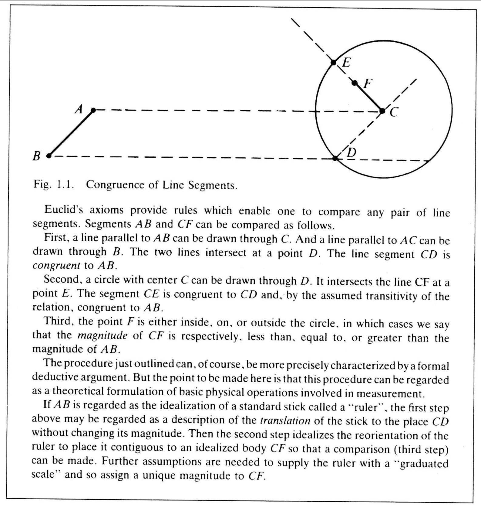
Fig. 1.1.

As Newton avers, geometry is the theory on which the practice of measurement is based. Geometrical figures can be regarded as idealizations of physical bodies. The theory of congruent figures is the central theme of geometry, and it provides a theoretical basis for measurement when it is regarded as an idealized description of the physical operations involved in classifying physical bodies according to size and shape (Figure 1.1). To put it another way, the theory of congruence specifies a set of rules to be used for classifying bodies. Apart from such rules the notions of size and shape have no meaning.

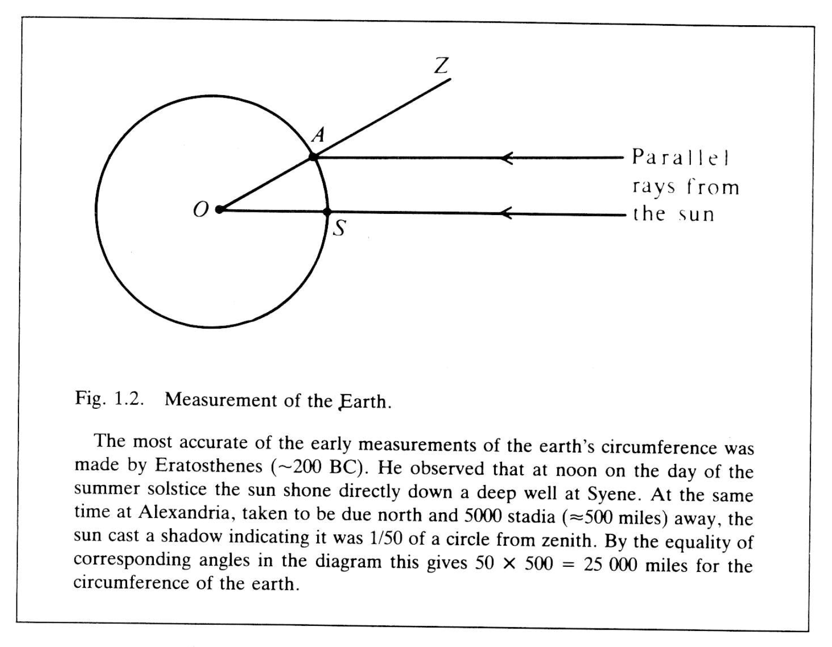
Fig. 1.2.

Greek geometry was certainly not developed with the problem of measurement in mind. Indeed, even the idea of measurement could not be conceived until geometry had been created. But already in Euclid’s day the Greeks had carried out impressive series of applications of geometry, especially to optics and astronomy (Figure 1.2), and this established a pattern to be followed in subsequent development of trigonometry and the practical art of measurement. With these efforts the notion of an experimental science began to take shape.

Today, “to measure” means to assign a number. But it was not always so. Euclid sharply distinguished “number” from “magnitude”. He associated the notion of number strictly with the operation of counting, so he recognized only natural numbers as numbers; even the notion of fraction as numbers had not yet been invented. For Euclid a magnitude was a segment. He frequently represented a whole number \, n \, by a line segment which is \, n \, times as long as some other line segment chosen to represent the number \, 1 . But he new that the opposite procedure is impossible, namely, that it is impossible to distinguish all line segments of different length by labeling them with numerals representing the counting numbers. He was able to prove this by showing that the side and the diagonal of a square cannot both be whole multiples of a single unit (Figure 1.3).

The “one way” correspondence of counting numbers with magnitudes shows that the latter concept is the more general of the two. With admirable consistency, Euclid carefully distinguished between the two concepts. This is born out by the fact that he proves many theorems twice , once for numbers and once for magnitudes. This rigid distinction between number and magnitude proved to be an impetus to progress in some direction, but an impediment to progress in others.

As in well known, even quite elementary problems lead to quadratic equations with solutions which are not integers or even rational numbers. Such problems have no solutions at all if only integers are recognized as numbers. The Hindus and the Arabs resolved this difficulty directly by generalizing the notion of number, but Euclid sidestepped it cleverly by reexpressing problems in arithmetic and algebra as problems in geometry. Then he solved for line segments instead as for numbers.

Thus, he represented the product \, x^2 \, as a square with a side of magnitude \, x . In fact, that is why we use the name “ \, x \, squared” today. The product \, x \, y \, was represented by a rectangle and called the “rectangle” of the two sides. The term “ \, x \, cubed”used even today originates from the representation of \, x^3 \, by a cube with side of magnitude \, x . But there are no corresponding representations of \, x^3 \, and higher powers of \, x \, in Greek geometry, so the Greek correspondence between algebra and geometry broke down. This “breakdown” impeded mathematical progress from antiquity until the seventeenth century, and its import is seldom recognized even today.

Commentators sometimes smugly dismiss Euclid’s practice of turning every algebra problem into an equivalent geometry problem as an inferior alternative to modern algebraic methods. But we shall find good reasons to conclude that, on the contrary, they have failed to grasp a subtlety of far-reaching significance in Euclid’s work. The real limitations on Greek mathematics were set by the failure of the Greeks to develop a simple symbolic language to express their profound ideas.

1-2. Number and Magnitude

The brilliant flowering of science and mathematics in ancient Greece was followed by a long period of scientific stagnation until an explosion of scientific knowledge in the seventeenth century gave birth to the modern world. To account for this explosion and its long delay after the impressive beginnings of science in Greece is one of the great problems in history. The “great man” theory implicit in so many textbooks would have us believe that the explosion resulted from the accidental birth of a cluster of geniuses like Kepler, Galileo and Newton. “Humanistic theories” attribute it to the social, political and intellectual climate of the Renaissance, stimulated by a rediscovery of the long lost culture of Greece. The invention and exploitation of the experimental method is a favorite explanation among philosophers and historians of science.

No doubt all these factors are important, but the most critical factor is often overlooked. The advances we know as modern science were not possible until an adequate number system had been created to express the results of measurement, and until a simple algebraic language had been invented to express relations among these results. While social and political disorders undoubtedly contributed to the decline of Greek culture, deficiences in the mathematical formalism of the Greek science must have been an increasingly powerful deterrent to every scientific advance and to the transmission of what had already been learned.

The long hiatus between Greek and Renaissance science is better regarded as a period of incubation instead of stagnation. For in this period the decimal system of arabic numerals was invented and algebra slowly developed. It can hardly be an accident that an explosion of scientific knowledge was ignited just as a comprehensive algebraic system began to take shape in the sixteenth and seventeenth centuries.

Though algebra was associated with geometry from its beginnings, René Descartes was the first to develop it systematically into a geometrical language. His first published work on the subject (1637) shows how clearly he had this objective in mind:

“Any problem in geometry can easily be reduced to such terms that a knowledge of the lengths of certain lines is sufficient for its construction. Just as arithmetic consists of only four or five operations, namely addition, subtraction, multiplication, division and the extraction of roots, which may be considered a kind of division, so in geometry, to find required lines it is merely necessary to add or subtract lines; or else, taking one line which I shall call unity in order to relate it as closely as possible to numbers, and which can in general be chosen arbitrarily, and having given two other lines, to find a fourth line which shall be to one of the given lines as the other is to unity (which is the same as multiplication); or, again to find a fourth line which is to one of the given lines as unity is to the other (which is equivalent to division); or, finally to find one, two, or several mean proportionals between unity and some other line (which is the same as extracting the square root, cube root, etc., of the given line). And I shall not hesitate to introduce these arithmetical terms into geometry, for the sake of greater clearness …”

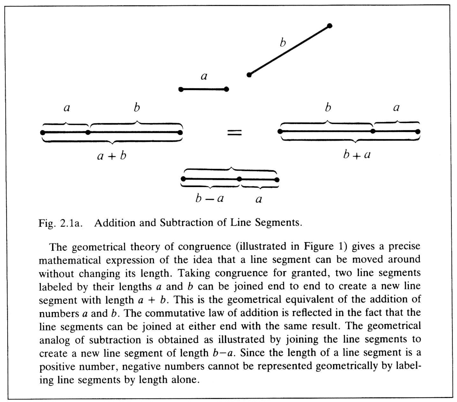
Fig. 2.1a.

Descartes gave the Greek notion of magnitude a happy symbolic form by assuming that every line segment can be uniquely represented by a number. He was the first person to label line segments by letters representing their numerical lengths. As he demonstrated, the aptness of this procedure resides in the fact that basic arithmetic operations such as addition and subtraction can be supplied with exact analogues in geometrical operations on line segments (Figures 2.1a, 2.1b).

One of his most significant innovations was to discard the Greek idea of representing the “product” of two line segments by a rectangle. In its stead he gave a rule for “multiplying” line segments which yielded another line segment in exact correspondence with the rule for multiplying numbers (Figure 2.2). This enabled him to avoid the apparent limitations of the Greek rule for “geometrical multiplication”.

Descartes could handle geometrical products of any order and he put this new ability to good use by showing how to use algebraic equations to describe geometric curves. This was the beginning of analytic geometry, and a crucial step in the development of the mathematical language that made significant improvements in algebraic notations, putting algebra in a form close to the one we use today.

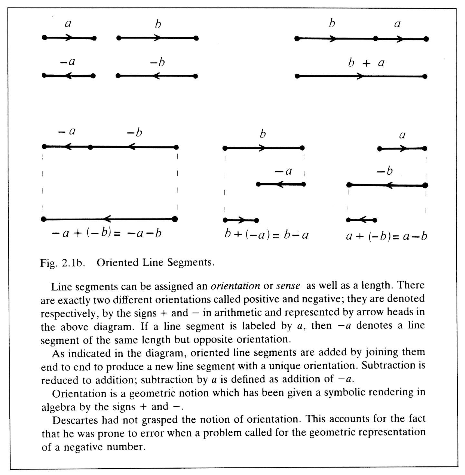
Fig. 2.1b.

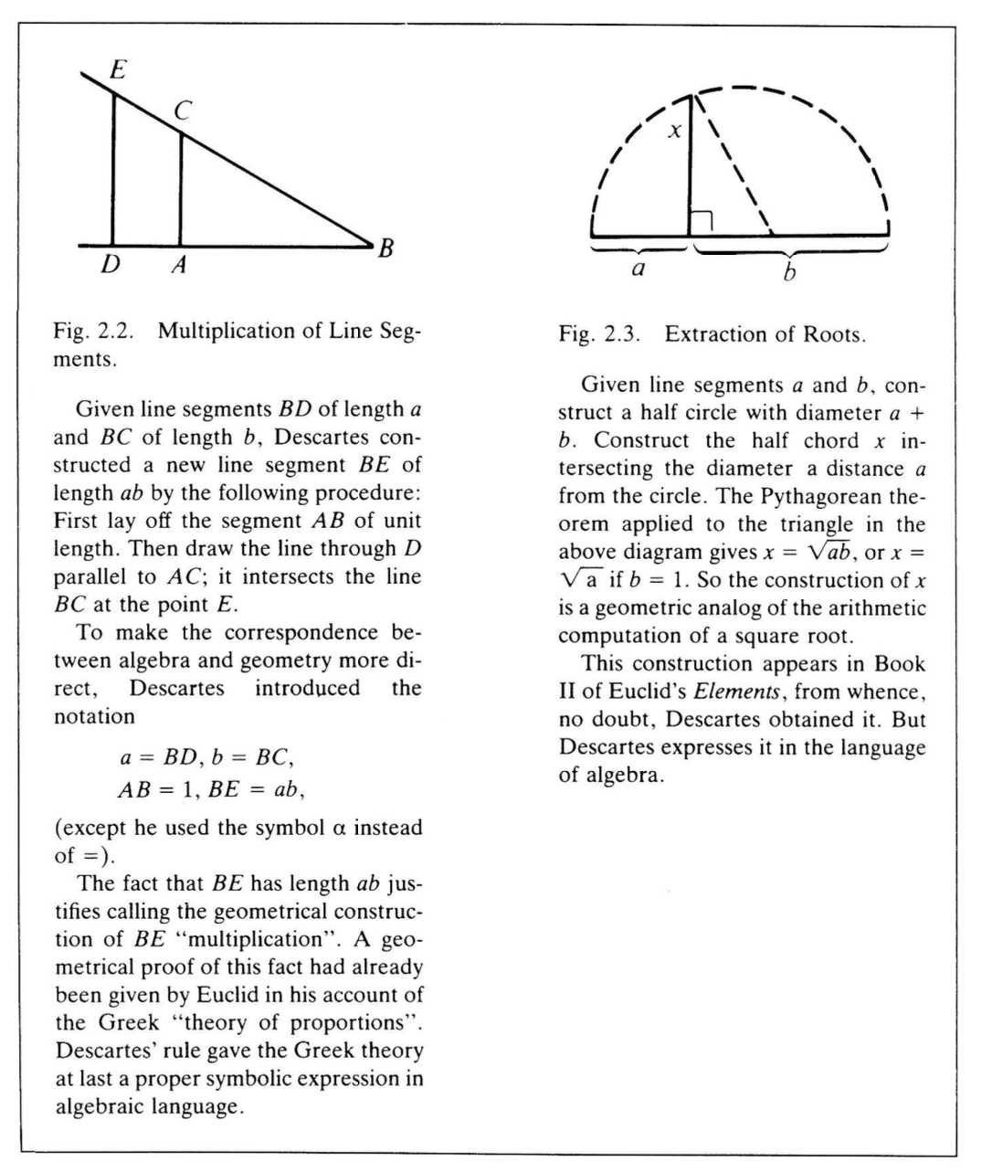
Fig. 2.2. and Fig. 2.3.

It has been said that the things a man takes for granted is a measure of his debt to his culture. The assumption of a complete correspondence between numbers and line segments was the foundation of Descartes’ union of geometry and algebra. A careful Greek logician like Eudoxus, would have demanded some justification for such a farreaching assumption. Yet, Descartes’ contemporaries accepted it without so much as a raised eyebrow. It did not seem revolutionary to them, because they were accustomed to it. In fact, algebra and arithmetic had never been free of some admixture of geometry. But a union could not be consummated until the notion of number and the symbolism of algebra had been developed to a degree consummate with Greek geometry. That state of affairs had just been reached when Descartes arrived on the historical scene.

Descartes stated explicitly what everyone had taken for granted. If Descartes had not done it someone else would have. Indeed, Fermat independently achieved quite similar results. But Descartes penetrated closer to the heart of the matter. His explicit union of number with the Greek geometric notion of magnitude sparked an intellectual explosion unequalled in all history.

Descartes was not in the habit of acknowledging his debt to others, but in a letter to Mersenne in 1637 he writes:

“As to the suggestion that what I have written could easily have been gotten from Vieta, the very fact that my treatise is hard to understand is due to my attempt to put nothing in it that I believed to be known either by him or by any one else…. I begin the rules of my algebra with what Vieta wrote at the very end of his book…. Thus, I began where he left off.”

The contribution of Vieta has been too frequently undervalued. He is the one who explicitly introduced the idea of using letters to represent constants as well as unknowns in algebraic equations. This act lifted algebra out of its infancy by separating the study of special properties of individual numbers from the abstract study of general properties of all numbers. It revealed the dependence of the number conept on the nature of algebraic operations.

Vieta used letters to denote numbers, and Descartes followed him by using letters to denote line segments. Vieta began the abstract study of rules for manipulating numbers, and Descartes pointed out the existence of similar rules for manipulating line segments Descartes gives some improvements on the symbolism and algebraic technique of Vieta, but it is hard to say how much of this that comes unacknowledged from the work of others. Before Vieta‘s innovations, the union of geometry and algebra could not have been effected.

The correspondence between numbers and line segments presumed by Descartes can be most simply expressed as the idea that numbers can be put into one to one correspondence with the points on a geometrical line (Figure 2.4). This idea seems to be nearly as old as the idea of a geometrical line itself. The Greeks may have believed it at first, but they firmly rejected it when incommensurables were discovered (Figure 1.3). Yet Descartes and his contemporaries evidently regarded it as obvious. Such a significant change in attitude must have an interesting history! Of course, such a change was possible only because the notion of number underwent a profound evolution.

Diophantus (250 AD), the last of the great Greek mathematicians, was probably the first to regard fractions as numbers. But the development most pertinent to the present discussion was the invention of algebraic numbers. This came about by presuming the existence of solutions to algebraic equations and devising symbols to represent them. Thus the symbol \, \sqrt 2 \, was invented to designate the solution to the equation \, x^2 = 2 \, . Once the symbol \, \sqrt 2 \, had been invented, it was hard to deny the reality of the number it names, and this number takes on a more concrete appearance when identified as the diagonal length of a unit square. In this way, the incommensurables of the Greeks received number names at last, and with no reason to the contrary, it must have seemed natural to assume that all points on a line can be named by numbers. So it seemed to Descartes. Perhaps it is a good thing that there was no latter-day Eudoxus to dampen Descartes’ ardor by proving that it is impossible to name every point on a line by an algebraic number. Descartes did not even suspect that the circumference of a unit circle is not an algebraic number, but then, that was not proved until 1882.

Deficiencies in the notion of number were not felt until the invention of calculus called for a clear idea of the “infinitely small”. A clear notion of “infinity” and with it a clear notion of the “continuum of real numbers” was not achieved until the latter part of the nineteenth century, when the real number system was “arithmeticized” by Weierstrass, Cantor and Dedekind. “Arithmeticize” means define the real numbers in terms of the natural numbers and their arithmetic, without appeal to any geometric intuition of “the continuum”. Some say that this development separated the notion of number from geometry. Rather the opposite is true. It consumated the union of number and geometry by establishing at last that the real numbers can be put into one to one correspondence with the points on a geometrical line. The arithmetical definition of the “real numbers” gave a precise symbolic expression to the intuitive notion of a continuous line (Figure 2.4).

Descartes began the explicit cultivation of algebra as a symbolic system for representing geometric notions. The idea of number has accordingly been generalized to make this possible. But the evolution of the number concept does not end with the invention of the real number system, because there is more to geometry than the linear continuum. In particular, the notions of direction and dimension cry out for a proper symbolic expression. The cry has been heard and answered.

1.3. Directed Numbers

After Descartes, the use of algebra as a geometric language expanded with ever mounting speed. So rapidly did success follow success in mathematics and in physics, so great was the algebraic skill that developed that for sometime no one noticed the serious limitations of this mathematical language.

Descartes expressed the geometry of his day in the algebra of his day. It did not occur to him that algebra could be modified to achieve a fuller symbolic expression in geometry. The algebra of Descartes could be used to classify line segments by length. But there is more to a line segment than length; it has direction as well. Yet the fundamental geometric notion of direction finds no expression in ordinary algebra. Descartes and his followers made up for this deficiency by augmenting algebra with the ever ready natural language. Expressions such as “the \, x -direction” and “the \, y -direction” are widely used even today. They are not part of the algebra, yet ordinary algebra cannot be applied to geometry without them.

Mathematics has steadily progressed by fashioning special symbolic systems to express ideas originally expressed in the natural language. The first mathematical system, Greek geometry, was formulated entirely in the natural language. How else was mathematics to start? But, to use the words of Descartes, algebra makes it possible to go “as far beyond the treatment of ordinary geometry, as the rhetoric of Cicero is beyond the a, b, c, of children”. How much more can be expected from further refinements of the geometrical language?

The generalization of number to incorporate the geometrical notion of direction as well as magnitude was not carried out until some two hundred years after Descartes. Though several people might be credited with conceiving the idea of “directed number“, Hermann Grassmann, in his book of 1844, developed this idea with a precision and completeness that far surpassed the work of anyone else at the time. Grassmann discovered a rule for relating line segments to numbers that differed slightly from the rule adopted by Descartes, and this led to a more general notion of number.

Before formulating the notion of a directed number, it is advantageous to substitute the short and suggestive word “scalar” for the more common but clumsy expression “real number“, and to recall the key idea of Descartes’ approach. Descartes unified algebra and geometry by corresponding the arithmetic of scalars with a kind of arithmetic of line segments. More specifically, if two line segments are congruent, that is, if one segment can be obtained from the other by translation and rotation, then Descartes would designate them by the same positive scalar. Conversely, every positive scalar designates an equivalence class of congruent line segments. This is the rule used by Descartes to relate numbers to line segments.

Alternatively, Grassmann chose to regard two line segments as “equivalent” if and only if one can be obtained from the other by translation; only then would he designate them by the same symbol. If a rotation was required to obtain one line segment from another, he regarded the line segments as “possessing different directions” and so designated them by different symbols. These conventions lead to the idea of “directed line segment” or vector, as a line segment which can be moved freely from place to place without changing either its magnitude or its direction. To achieve a simple symbolic expression of this idea and yet distinguish vectors from scalars, vectors will be represented by letters in bold face type. If two directed line segments designated by vectors \, \bold a \, and \, \bold b \, respectively, have the same magnitude and direction, then the vectors are said to be equal, and, as in scalar algebra, one writes

\, \bold a = \bold b \;\;\;\;\;\;\;\;\;\;\;\;\;\;\;\;\;\;\;\;\;\;\;\;\;\;\;\;\;\;\;\;\;\;\;\;\;\;\;\;\;\;\;\;\;\;\;\;\;\;\;\;\;\;\;\;\;\;\;\;\;\;\;\;\;\;\;\;\;\;\;\;\;\;\;\;\;\;\;\;\;\;\;\;\;\;\;\;\;\;\; (3.1)

Of course the use of vectors to express the geometrical fact that line segments may differ in direction does not obviate the value of classifying line segments by length. But a simple formulation of the relation between scalars and vectors is called for. It can be achieved by observing that to every vector \, \bold a \, there corresponds a unique positive scalar, here denoted by \, | \bold a | \, and called the “magnitude” or the “length” of \, \bold a . This follows from the correspondence between scalars and line segments which has already been discussed.

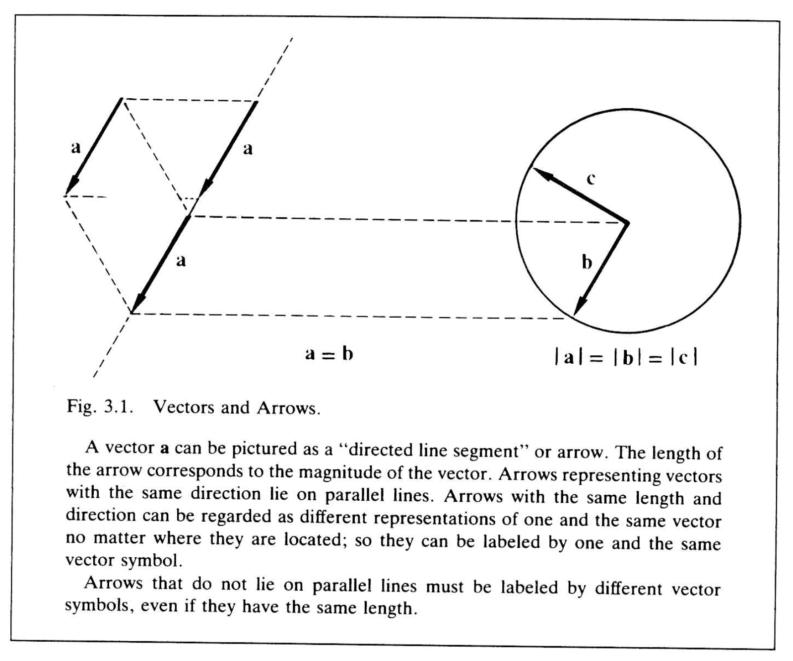
Fig. 3.1.

Suppose, now, that a vector \, \bold b \, has the same direction as \, \bold a , but \, | \bold b | = \lambda | \bold a | , where \, \lambda \, is a positive scalar. This can be expressed simply by writing

\, \bold b = \lambda \bold a \;\;\;\;\;\;\;\;\;\;\;\;\;\;\;\;\;\;\;\;\;\;\;\;\;\;\;\;\;\;\;\;\;\;\;\;\;\;\;\;\;\;\;\;\;\;\;\;\;\;\;\;\;\;\;\;\;\;\;\;\;\;\;\;\;\;\;\;\;\;\;\;\;\;\;\;\;\;\;\;\;\;\;\;\;\;\;\;\; (3.2)

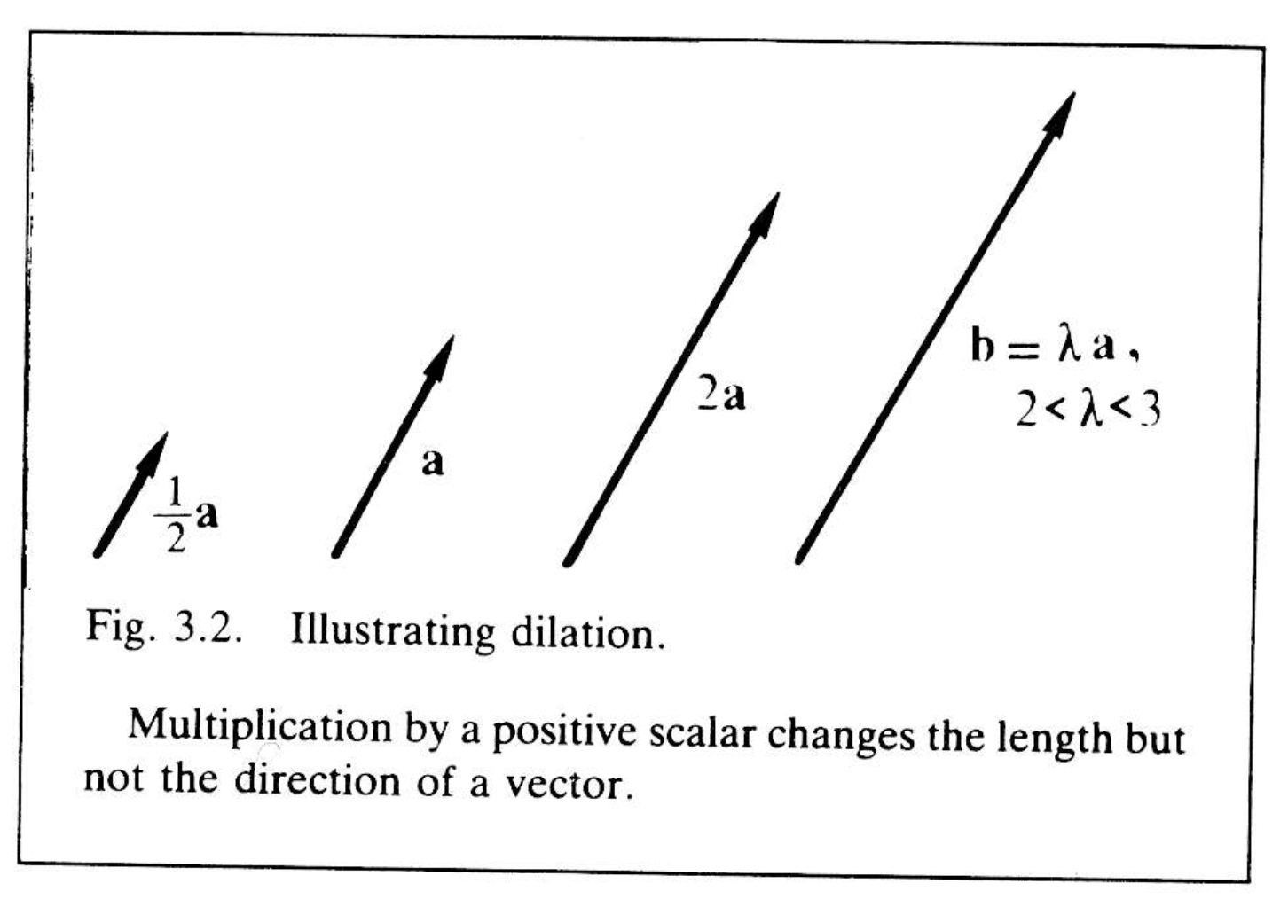
Fig. 3.2.

But this can be interpreted as an equation defining the multiplication of a vector by a scalar. Thus, multiplication by a positive scalar changes the magnitude of a vector but not its direction (Figure 3.2). This operation is commonly called a dilation.

If \, \lambda > 1 \, , it is an expansion, since then \, | \, \bold b \, | > | \, \bold a \, | , and if \, \lambda < 1 , it is a contraction, since then \, | \, \bold b \, | < | \, \bold a \, | . Descartes’ geometrical construction for “multiplying” two line segments (Figure 2.2) is a dilation of one segment by the magnitude of the other. Equation (3.2) allows one to write \, \bold a = | \, \bold a \, | \, \bold {â} , where

| \, \bold {â} \, | = 1. \;\;\;\;\;\;\;\;\;\;\;\;\;\;\;\;\;\;\;\;\;\;\;\;\;\;\;\;\;\;\;\;\;\;\;\;\;\;\;\;\;\;\;\;\;\;\;\;\;\;\;\;\;\;\;\;\;\;\;\;\;\;\;\;\;\;\;\;\;\;\;\;\;\;\;\;\;\;\;\;\;\;\;\;\;\; (3.3)

This expresses the vector \, \bold a \, as the product of its magnitude \, | \, \bold a \, | with a “unit vector” \, \bold {â} . The “unit” \, \bold {â} \, uniquely specifies the direction of \, \bold a \, , so Equation (3.3) can be regarded as a decomposition of \, \bold a \, into magnitude and direction. If Equation (3.2) is supposed to hold, then multiplication of a vector \, \bold a \, by zero results in a vector with zero magnitude. This can be expressed by writing

\, (0) \, \bold a = 0. \;\;\;\;\;\;\;\;\;\;\;\;\;\;\;\;\;\;\;\;\;\;\;\;\;\;\;\;\;\;\;\;\;\;\;\;\;\;\;\;\;\;\;\;\;\;\;\;\;\;\;\;\;\;\;\;\;\;\;\;\;\;\;\;\;\;\;\;\;\;\;\;\;\;\;\;\;\;\;\;\;\;\;\;\; (3.4)

Since the direction associated with a line segment of zero length seems to be of no consequence, it is natural to assume that the zero vector on the right side of (3.4) is a unique number no matter what the direction of \, \bold a . Moreover, it will be seen later that there is good reason to regard the zero vector as one and the same number as the zero scalar. So the zero on the right side of (3.4) is not written in bold face type. Grassmann may have been the first person to clearly understand that the significance of a number lies not in itself but solely in its relations to other numbers. The notion of number resides in the rules for combining two numbers to get a third. Grassmann looked for rules for combining vectors which would fully describe the geometrical properties of directed line segments. He noticed that two directed line segments connected end to end determined a third, which may be regarded as their sum. This “geometrical sum” of directed line segments can be simply represented by an equation for corresponding vectors \, \bold a , \, \bold b \, , \, \bold s :

\, \bold a + \bold b = \bold s. \;\;\;\;\;\;\;\;\;\;\;\;\;\;\;\;\;\;\;\;\;\;\;\;\;\;\;\;\;\;\;\;\;\;\;\;\;\;\;\;\;\;\;\;\;\;\;\;\;\;\;\;\;\;\;\;\;\;\;\;\;\;\;\;\;\;\;\;\;\;\;\;\;\;\;\;\;\;\;\;\;\;\;\; (3.5)

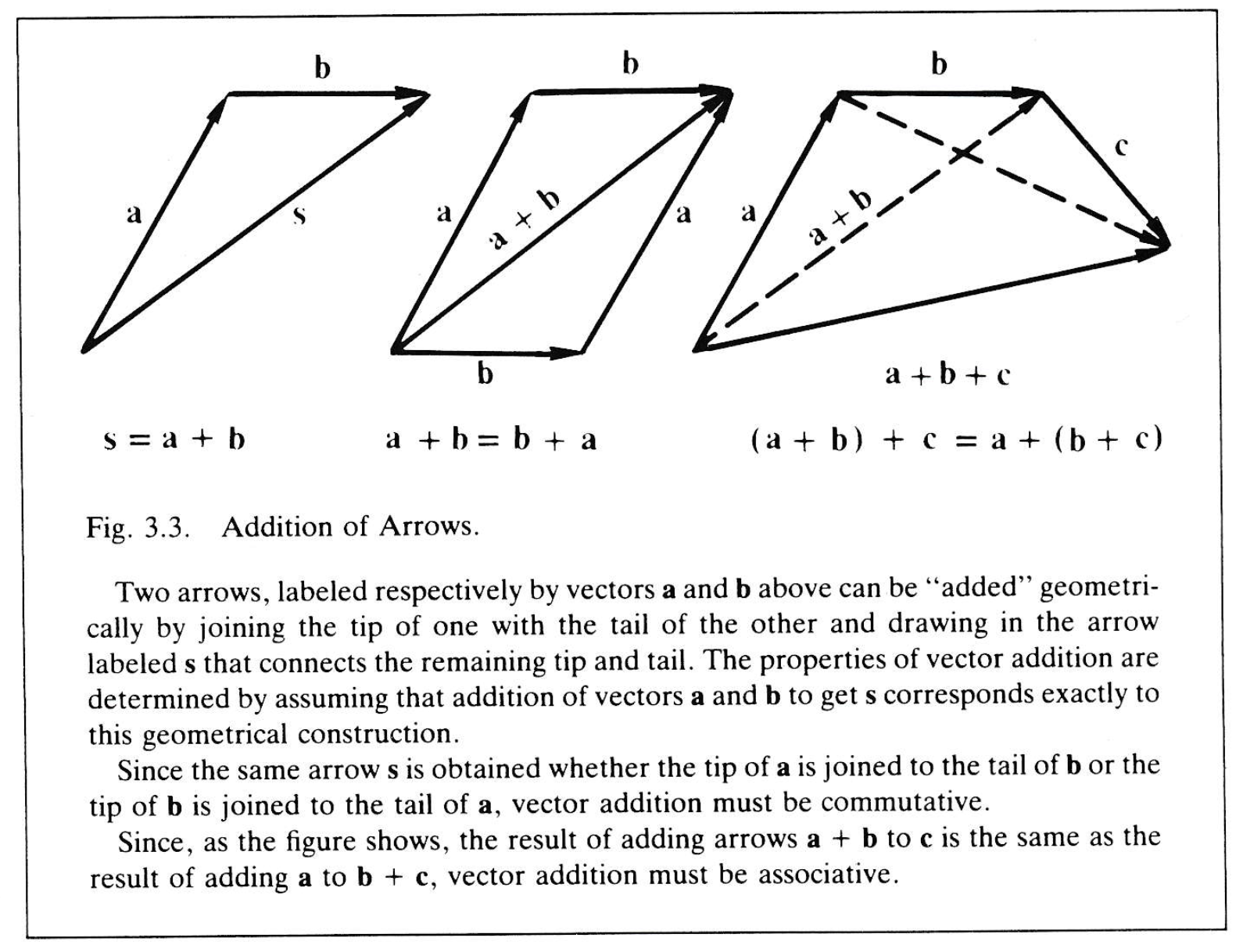
Fig. 3.3.

This procedure is like the one used by Descartes to relate “geometrical addition of line segments” to addition of scalars, except that the definition of “geometrically equivalent” line segments is different.

The rules for adding vectors are determined by the assumed correspondence with directed line segments. As shown in Figure 3.3, vector addition, like scalar addition, must obey the commutative rule.

\, \bold a + \bold b = \bold b + \bold a, \;\;\;\;\;\;\;\;\;\;\;\;\;\;\;\;\;\;\;\;\;\;\;\;\;\;\;\;\;\;\;\;\;\;\;\;\;\;\;\;\;\;\;\;\;\;\;\;\;\;\;\;\;\;\;\;\;\;\;\;\;\;\;\;\;\;\;\;\;\;\;\;\;\;\;\;\;\; (3.6)

and the associative rule,

\, ( \bold a + \bold b ) + \bold c = \bold a + ( \bold b + \bold c ). \;\;\;\;\;\;\;\;\;\;\;\;\;\;\;\;\;\;\;\;\;\;\;\;\;\;\;\;\;\;\;\;\;\;\;\;\;\;\;\;\;\;\;\;\;\;\;\;\;\;\;\;\;\;\;\;\;\;\;\; (3.7)

As in scalar algebra, the number zero plays a special role in vector addition. Thus,

\, \bold a + 0 = \bold a. \;\;\;\;\;\;\;\;\;\;\;\;\;\;\;\;\;\;\;\;\;\;\;\;\;\;\;\;\;\;\;\;\;\;\;\;\;\;\;\;\;\;\;\;\;\;\;\;\;\;\;\;\;\;\;\;\;\;\;\;\;\;\;\;\;\;\;\;\;\;\;\;\;\;\;\;\;\;\;\;\;\;\;\;\; (3.8)

Moreover, to every vector \, \bold a \, there corresponds one and only one vector \, \bold b \, which satisfies the equation

\, \bold a + \bold b = 0. \;\;\;\;\;\;\;\;\;\;\;\;\;\;\;\;\;\;\;\;\;\;\;\;\;\;\;\;\;\;\;\;\;\;\;\;\;\;\;\;\;\;\;\;\;\;\;\;\;\;\;\;\;\;\;\;\;\;\;\;\;\;\;\;\;\;\;\;\;\;\;\;\;\;\;\;\;\;\;\;\;\;\;\;\; (3.9)

This unique vector is called the negative of \, \bold a \, and denoted by \, - \bold a \, (Figure 3.4).

The existence of negatives makes it possible to define subtraction as addition of a negative. Thus,

\, \bold c - \bold a \, \stackrel {\mathrm{def}}{=} \, \bold b + ( - \bold a ). \;\;\;\;\;\;\;\;\;\;\;\;\;\;\;\;\;\;\;\;\;\;\;\;\;\;\;\;\;\;\;\;\;\;\;\;\;\;\;\;\;\;\;\;\;\;\;\;\;\;\;\;\;\;\;\;\;\;\;\;\;\;\;\;\;\;\;\;\;\; (3.10)

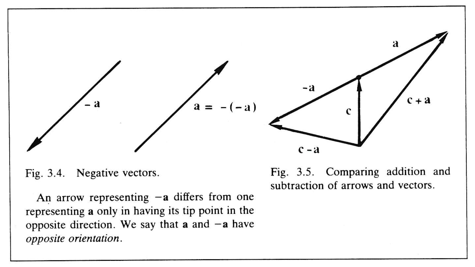
Fig. 3.4. and Fig. 3.5.

Subtraction and addition are compared in Figure 3.5.

The existence of negatives also makes it possible to define multiplication by the scalar \, -1 \, by the equation

\, (-1) \bold a \, \stackrel {\mathrm{def}}{=} \, - \bold a. \;\;\;\;\;\;\;\;\;\;\;\;\;\;\;\;\;\;\;\;\;\;\;\;\;\;\;\;\;\;\;\;\;\;\;\;\;\;\;\;\;\;\;\;\;\;\;\;\;\;\;\;\;\;\;\;\;\;\;\;\;\;\;\;\;\;\;\;\;\;\;\;\;\;\;\;\;\; (3.11)

This operation justifies interpreting \, -1 \, as a representation of the operation of reversing direction (i.e. orientation, as explained in Figure 2.1B). Then the equation \, {(-1)}^2 = 1 \, simply expresses the obvious geometrical fact that by reversing direction twice one reproduces the original direction. In this way the concept of directed numbers leads to an operational interpretation of negative numbers.

Now that the geometrical meaning of multiplication by minus one is understood, it is obvious that Equation (3.2) is meaningful even if \, \lambda \, is a negative scalar. Vectors which are scalar multiples of one another are said to be codirectional or collinear.

1-4. The Inner Product

A great many significant geometrical theorems can be simply expressed and proved with the algebraic rules for vector addition and scalar multiplication which have just been set down. However, the algebraic system as it stands cannot be regarded as a complete symbolic expression of the geometric notions of magnitude and direction, because if fails to fully indicate the difference between scalars and vectors. This difference is certainly not reflected in the rules for addition, which are the same for both scalars and vectors. In fact, the distinction between scalars and vectors still resides only in their geometric interpretations, that is, in the different rules used to correspond them with line segments.

The opportunity to give the notion of direction a full algebraic expression arises when the natural question of how to multiply vectors is entertained. Descartes gave a rule for “multiplying” line segments, but this rule does not depend on the direction of the line segments, and it already has an algebraic interpretation as a dilation. Yet, the general approach of Descartes can be followed to a different end.

One can look for a significant geometrical construction based on two line segments that does depend on direction; then, by correspondence, use this construction to define the product of two vectors.

One need not look far, for one of the most familiar constructions of ordinary geometry is readily seen to meet the desired specifications, namely the perpendicular projection of one line segment onto another. (Figure 4.1). A study of this construction reveals that, though it depends on the relative directions of the line segments to be “multiplied”, the result depends on the magnitude of only one of them. This result can be multiplied by the magnitude of the other to get a more symmetrical relation. In this way one is led to the following rule for multiplying vectors:

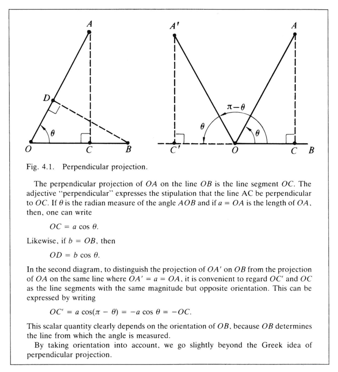
Fig. 4.1.

Define the inner product of two directed line segments, denoted by vectors \, \bold a \, and \, \bold b \, respectively, to be the oriented line segment obtained by dilating the projection of \, \bold a \, onto \, \bold b \, by the magnitude of \, \bold b .

The magnitude and the orientation of the resulting line segment is a scalar; denote this scalar by \, \bold a \cdot \bold b \, and call it the inner product of vectors \, \bold a \, and \, \bold b .

This definition of \, \bold a \cdot \bold b \, implies the following relation to the angle \, \theta \, between \, \bold a \, and \, \bold b :

\, \bold a \cdot \bold b = | \, \bold a \, | \, | \, \bold b \, | \, \cos \theta. \;\;\;\;\;\;\;\;\;\;\;\;\;\;\;\;\;\;\;\;\;\;\;\;\;\;\;\;\;\;\;\;\;\;\;\;\;\;\;\;\;\;\;\;\;\;\;\;\;\;\;\;\;\;\;\;\;\;\;\;\;\;\;\;\;\;\;\;\; (4.1)

This expression is commonly taken as the definition of \, \bold a \cdot \bold b , but that calls for an independent definition of \, \cos \theta , which would be out of place here.

It should be noted that the geometrical construction on which the definition of \, \bold a \cdot \bold b \, is based actually gives a line segment directed along the same line as \, \bold a \, or \, \bold b ; the magnitude and the relative orientation of this line segment were used in the definition of \, \bold a \cdot \bold b \, but its direction was not.

There is good reason for this. It is necessary if the algebraic rule for multiplication is to depend only on the relative directions of \, \bold a \, and \, \bold b . Thus, as defined, the numerical value of \, \bold a \cdot \bold b \, is unaffected by any change in the directions of \, \bold a \, and \, \bold b \, which leaves the angle between \, \bold a \, and \, \bold b \, fixed. Moreover, \, \bold a \cdot \bold b \, has the important symmetry property

\, \bold a \cdot \bold b = \bold b \cdot \bold a. \;\;\;\;\;\;\;\;\;\;\;\;\;\;\;\;\;\;\;\;\;\;\;\;\;\;\;\;\;\;\;\;\;\;\;\;\;\;\;\;\;\;\;\;\;\;\;\;\;\;\;\;\;\;\;\;\;\;\;\;\;\;\;\;\;\;\;\;\;\;\;\;\;\;\;\;\;\;\;\;\;\; (4.2)

This expresses the fact that the projection of \, \bold a \, onto \, \bold b \, dilated by \, | \, \bold b \, | \, gives the same result as the projection of \, \bold b \, onto \, \bold a \, dilated by \, | \, \bold a \, | \, (Figure 4.2)

The inner product has, besides (4.2), several basic algebraic properties which can easily be deduced from its definition by correspondence with perpendicular projection. Its relation to scalar multiplication of vectors is expressed by the rule

\,( \lambda \, \bold a ) \cdot \bold b = \lambda (\bold a \cdot \bold b) = \bold a \cdot ( \lambda \, \bold b). \;\;\;\;\;\;\;\;\;\;\;\;\;\;\;\;\;\;\;\;\;\;\;\;\;\;\;\;\;\;\;\;\;\;\;\;\;\;\;\;\;\;\;\;\;\;\;\;\;\;\;\;\;\; (4.3)

Here \, \lambda \, can be any scalar – positive, negative or zero. Its relation to vector addition is expressed by the distributive rule

\, \bold a \cdot ( \bold b + \bold c ) = \bold a \cdot \bold b + \bold a \cdot \bold c. \;\;\;\;\;\;\;\;\;\;\;\;\;\;\;\;\;\;\;\;\;\;\;\;\;\;\;\;\;\;\;\;\;\;\;\;\;\;\;\;\;\;\;\;\;\;\;\;\;\;\;\;\;\;\;\;\;\;\;\;\; (4.4)

(Figure 4.3). The magnitude of a vector is related to the inner product by

\, \bold a \cdot \bold a = {| \,\bold a \, |}^2 ≥ 0. \;\;\;\;\;\;\;\;\;\;\;\;\;\;\;\;\;\;\;\;\;\;\;\;\;\;\;\;\;\;\;\;\;\;\;\;\;\;\;\;\;\;\;\;\;\;\;\;\;\;\;\;\;\;\;\;\;\;\;\;\;\;\;\;\;\;\;\;\;\;\;\;\;\;\; (4.5)

Of course, \, \bold a \cdot \bold a = 0 \, if and only if \, \bold a = 0 .

The inner product greatly increases the usefulness of vectors, for it can be used to compute angles and the lengths of line segments. Important theorems of geometry and trigonometry can be proved easily by the methods of “vector algebra”, so easily, in fact, that it is hardly necessary to single them out by calling them theorems. Results which men once went to great pains to prove have been worked into the algebraic rules where they can be exploited routinely. For example, everyone knows that a great many theorems about triangles are proved in trigonometry and geometry. But, such theorems seem superfluous when it is realized that a triangle can be completely characterized by the simple vector equation

\, \bold a + \bold b = \bold c. \;\;\;\;\;\;\;\;\;\;\;\;\;\;\;\;\;\;\;\;\;\;\;\;\;\;\;\;\;\;\;\;\;\;\;\;\;\;\;\;\;\;\;\;\;\;\;\;\;\;\;\;\;\;\;\;\;\;\;\;\;\;\;\;\;\;\;\;\;\;\;\;\;\;\;\;\;\;\;\;\;\;\;\; (4.6)

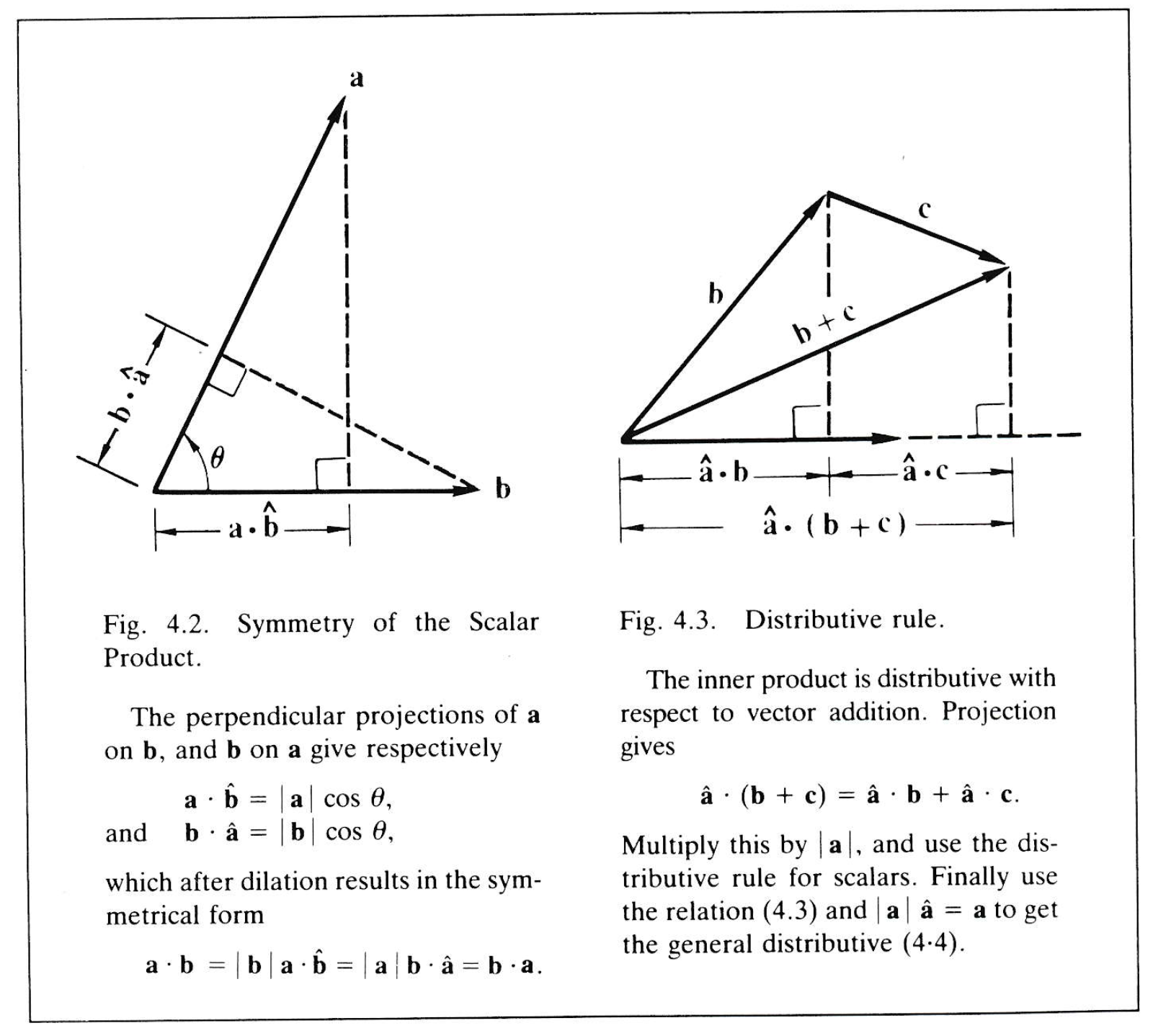
Fig. 4.2 and Fig. 4.3.

From this equation various properties of a triangle can be derived by simple steps. For instance, by “squaring” and using the distributive rule (4.4) one gets an equation relating sides and angles:

\, \bold c \cdot \bold c \, = \, ( \bold a + \bold b ) \cdot ( \bold a + \bold b )
\;\;\;\;\;\;\;\; \, = \, \bold a \cdot ( \bold a + \bold b ) + \bold b \cdot ( \bold a + \bold b )
\;\;\;\;\;\;\;\; \, = \, \bold a \cdot \bold a + \bold b \cdot \bold b + \bold a \cdot \bold b + \bold b \cdot \bold a.

Or, using (4.2) and (4.5),

\, {| \, \bold c \, |}^{\, 2} = {| \, \bold a \, |}^{\, 2} + {| \, \bold b \, |}^{\, 2} + 2 \, \bold a \cdot \bold b. \;\;\;\;\;\;\;\;\;\;\;\;\;\;\;\;\;\;\;\;\;\;\;\;\;\;\;\;\;\;\;\;\;\;\;\;\;\;\;\;\;\;\;\;\;\;\;\;\;\;\;\; (4.7)

This equation can be reexpressed in terms of scalar labels still commonly used in trigonometry. Figure 4.4 indicates the relations

\, a = | \, \bold a \, | , \, b = | \, \bold b \, | \, , \, \bold a \cdot \bold b = - a \, b \, \cos C .

So (4.7) can be written in the form

\, c^2 = a^2 + b^2 + 2 \, a \, b \, \cos C. \;\;\;\;\;\;\;\;\;\;\;\;\;\;\;\;\;\;\;\;\;\;\;\;\;\;\;\;\;\;\;\;\;\;\;\;\;\;\;\;\;\;\;\;\;\;\;\;\;\;\;\;\;\;\;\;\;\; (4.8)

This formula is called the “law of cosines” in trigonometry. If \, C \, is a right angle, then \, \cos C = 0 , and Equation (4.8) reduces to the Pythagorean Theorem.

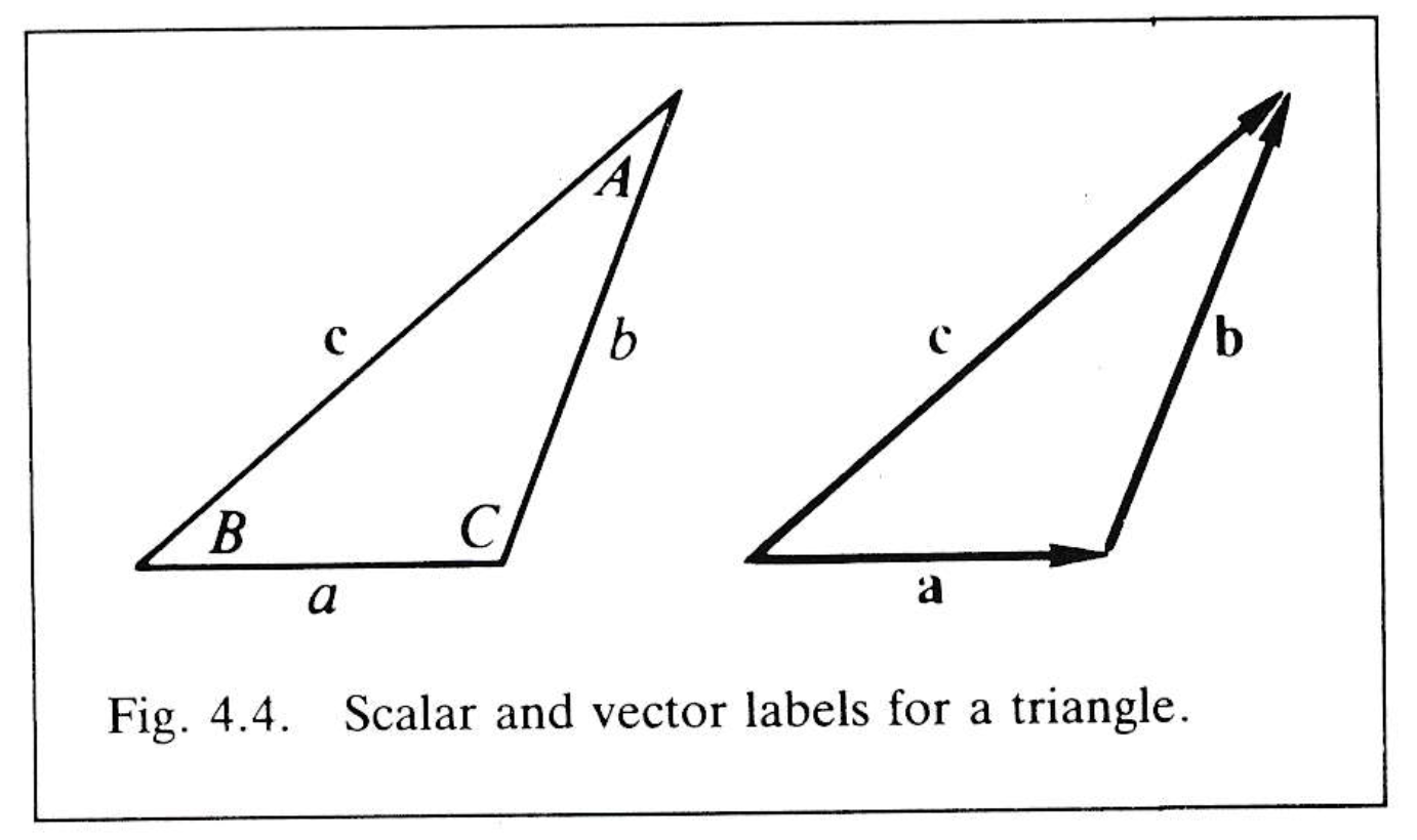
Fig. 4.4.

By rewriting (4.6) in the form \, \bold a = \bold c - \bold b \, and squaring one gets a formula similar to (4.8) involving the angle \, A . Similarly, an equation involving angle \, B \, can be obtained. In this way one gets three equations relating the scalars \, a, b, c, A, B, C . These equations show that given the magnitude of the three sides, or of two sides and the angle between, the remaining three scalars can be computed. This result may be recognized as encompassing several theorems of geometry. The point to be made here is that these results of geometry and trigonometry need not be remembered as theorems, since they can be obtained so easily by the “algebra” of scalars and vectors.

Trigonometry is founded on the Greek theories of proportion and perpendicular projection. But the principle ideas of trigonometry did not find their simplest symbolic expression until the invention of vectors and the inner product by Grassmann. Grassmann originally defined the inner product just as we did by correspondence with a perpendicular projection. But he also realized that once the basic algebraic properties have been determined by correspondence, no further reference to the idea of projection is necessary. Thus the “inner product” can be fully defined abstractly as a rule relating scalars to vectors which has the properties specified by Equations (4.2) through (4.5).

With the abstract definition of \, \bold a \cdot \bold b \, the intuitive notion of relative direction at last receives a precise symbolic formulation. The notion of number is thereby nearly developed to the point where the principles and theorems of geometry can be completely expressed by algebraic equations without the need to use natural language. For example, the statement “lines \, OA \, and \, OB \, are perpendicular” can now be better expressed by the equation

\, \bold a \cdot \bold b \, = \, 0. \;\;\;\;\;\;\;\;\;\;\;\;\;\;\;\;\;\;\;\;\;\;\;\;\;\;\;\;\;\;\;\;\;\;\;\;\;\;\;\;\;\;\;\;\;\;\;\;\;\;\;\;\;\;\;\;\;\;\;\;\;\;\;\;\;\;\;\;\;\;\;\;\;\;\;\;\;\;\;\;\;\;\;\;\; (4.9)

Trigonometry can now be regarded as a system of algebraic equations and relations without any mention of triangles and projections. However, it is precisely the relations of vectors to triangles and of the inner product to projections that makes the algebra of scalars and vectors a useful language for describing the real world. And that, after all, is what the whole scheme was designed for.

1-5. The Outer Product

The algebra of scalars and vectors based on the rules just mentioned has been so widely accepted as to be routinely employed by mathematicians and physicists today. As it stands, however, this algebra is still incapable of providing a full expression of geometrical ideas. Yet there is nothing close to consensus on how to overcome this limitation.

Rather there is a great proliferation of different mathematical systems designed to express geometrical ideas – tensor algebra, matrix algebra, spinor algebra – to name just a few of the most common. It might be thought that this profusion of systems reveals the richness of mathematics. On the contrary, it reveals the widespread confusion – confusion about the aims and principles of geometric algebra. the intent here is to clarify these aims and principles by showing that the preceeding arguments leading to the invention of scalars and vectors can be continued in a natural way, culminating in a single mathematical system which facilitates a simple expression of the full range of geometrical ideas.

The principle that the product of two vectors ought to describe their relative directions presided over the definition of the inner product. But the inner product falls short of a complete fulfillment of that principle, because it fails to express the fundamental geometrical fact that two non-collinear directed line segments determine a parallelogram. The possibility of giving this important feature of geometry a direct algebraic expression becomes apparent when the parallelogram is regarded as a kind of “geometric product” of its sides. But to make this possibility a reality, the notion of number must be generalized.

A parallelogram can be regarded as a directed plane segment. Just as vectors were invented to characterize the notion of a directed line segment, so a new kind of directed number, called a bivector or 2-vector, can be introduced to characterize the notion of a directed plane segment (Figure 5.1).

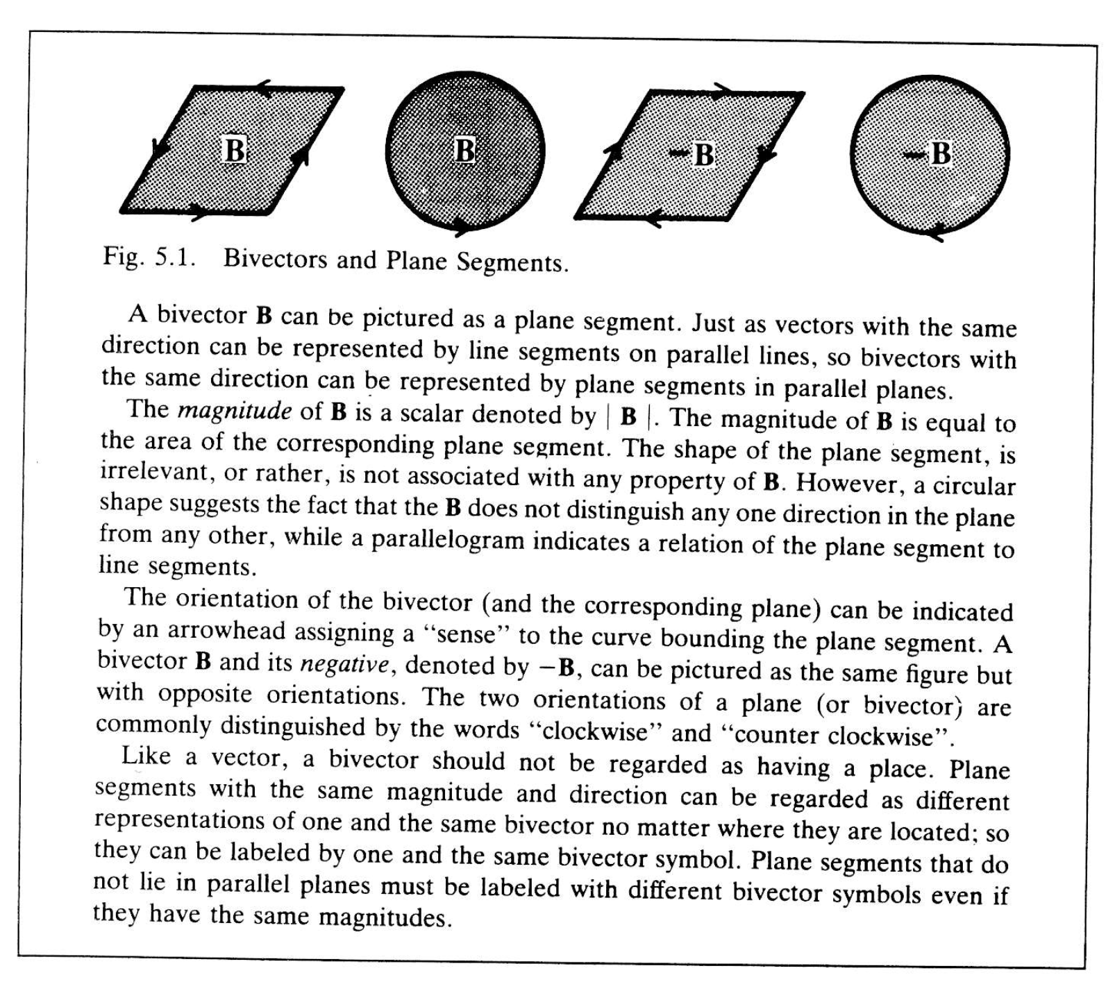
Fig. 5.1.

Like a vector, a bivector has magnitude, direction, and orientation, and only these properties. But here the word “direction” must be understood in a sense more general than is usual. Just as the direction of a vector corresponds to an (oriented straight) line, so the direction of a bivector corresponds to an (oriented flat) plane. The distinction between these two kinds of direction involves the geometrical notion of dimension or grade.

Accordingly, the direction of a bivector is said to be 2-dimensional to distinguish it from the 1-dimensional direction of a vector. And it is sometimes convenient to call a vector a 1-vector to emphasize its dimension. Also, a scalar can be regarded as a 0-vector, to indicate that it is a 0-dimensional number. Since, as already shown, the only directional property of a scalar is its orientation, orientation can be regarded as a 0-dimensional direction. Thus the idea of numbers with different geometrical dimension begins to take shape.

In ordinary geometry the concepts of line and plane play roles of comparable significance. Indeed, the one concept can hardly be said to have any significance at all apart from the other, and the mathematical meanings of”line” and “plane” are determined solely by specifying relations between them. To give “planes” and “lines” equal algebraic representations, the notions of directed number must be enlarged to include the notion of of bivector as well as vector, and the relations of lines to planes must be reflected in the relations of vectors to bivectors.

It may be a good idea to point out that both line and plane, as commonly conceived, consist of a set of points in definite relation to one another. It is the nature of this relation that distinguishes line from plane. A single vector completely characterizes the directional relation of points in a given line. A single bivector completely characterizes the directional relation of points in a given plane. In other words, a bivector does not describe a set of points in a plane, rather it describes the directional property of such a set, which, so to speak, specifies the plane the points are “in”. Thus, the notion of a plane as a relation can be separated from the notion of a plane as a point set. After the directional properties of planes and lines have been fully incorporated into an algebra of directed numbers, the geometrical properties of point sets can be more easily and completely described than ever before, as we shall see.

Now return to the problem of giving algebraic expression to the relation of line segments to plane segments. Note that a point moving a distance and direction specified by a vector \, \bold a \, sweeps out a directed line segment. And the points on this line segment, each moving a distance and direction specified by a vector \, \bold b \, sweeps out a parallelogram, (Figure 5.2). Since the bivector \, \bold B \, corresponding to this parallelogram is clearly uniquely determined by this geometrical construction, it may be regarded as a kind of “product” of the vectors \, \bold a \, and \, \bold b . So write

\, \bold a \wedge \bold b \, = \, \bold B. \;\;\;\;\;\;\;\;\;\;\;\;\;\;\;\;\;\;\;\;\;\;\;\;\;\;\;\;\;\;\;\;\;\;\;\;\;\;\;\;\;\;\;\;\;\;\;\;\;\;\;\;\;\;\;\;\;\;\;\;\;\;\;\;\;\;\;\;\;\;\;\;\;\;\;\;\;\;\;\;\;\; (5.1)

A “wedge” is used to denote this new kind of multiplication to distinguish it from the “dot” denoting the inner product of vectors. The bivector \, \bold a \wedge \bold b \, is said to be the outer product of vectors \, \bold a \, and \, \bold b .

Fig. 5.2.

Now note that the parallelogram obtained by “ \, \bold b \, along \, \bold a \, ” differs only in orientation from the parallelogram obtained by “sweeping \, \bold a \, along \, \bold b \, (Figure 5.2). This can be simply expressed by writing

\, \bold b \wedge \bold a \, = \, - \bold a \wedge \bold b \, = - \bold B. \;\;\;\;\;\;\;\;\;\;\;\;\;\;\;\;\;\;\;\;\;\;\;\;\;\;\;\;\;\;\;\;\;\;\;\;\;\;\;\;\;\;\;\;\;\;\;\;\;\;\;\;\;\;\;\;\;\;\;\;\;\; (5.2)

Thus, reversing the order of vectors in an outer product “reverses” the orientation of the resulting bivector. This is expressed by saying that the outer product is anticommutative.

The relation of vector orientation to bivector orientation is fixed by the rule

\, \bold b \wedge \bold a \, = \, \bold a \wedge (-\bold b) \, = (- \bold b) \wedge (-\bold a) \, = \, (- \bold a) \wedge \bold b. \;\;\;\;\;\;\;\;\;\;\;\;\;\;\;\;\;\;\;\;\;\;\;\;\; (5.3)

This rule, like the others, follows from the correspondence of vectors and bivectors with oriented line segments and plane segments. It can be simply “read off” from Figure 5.3.

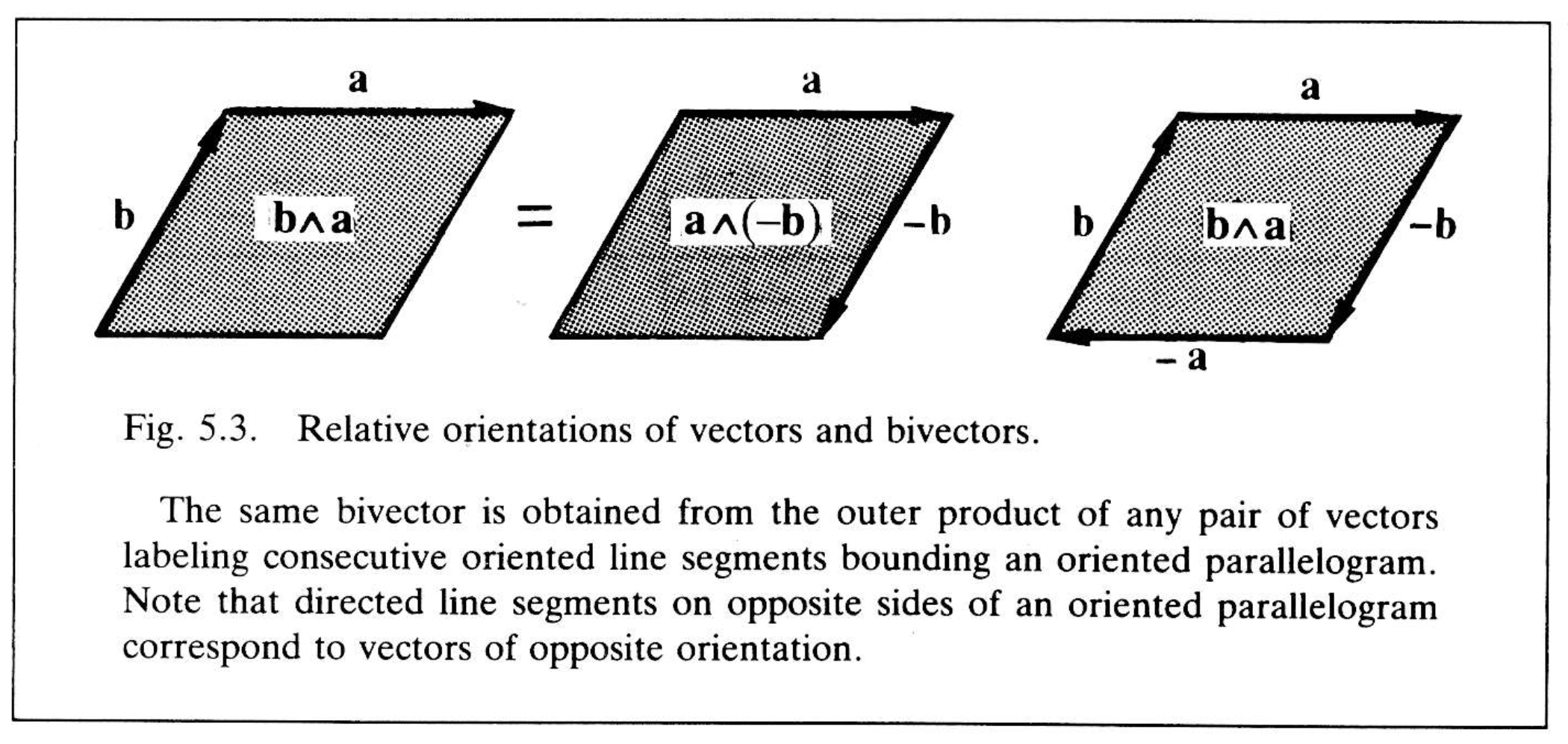
Fig. 5.3.

Since the magnitude of the bivector \, \bold a \wedge \bold b \, is just the area of the corresponding parallelogram,

\, | \, \bold B \, | \, = \, | \, \bold a \wedge \bold b \, | \, = \, | \, \bold b \wedge \bold a \, | \, = | \, a \, | \, | \,| \, b \, | \, \sin \theta. \;\;\;\;\;\;\;\;\;\;\;\;\;\;\;\;\;\;\;\;\;\;\;\;\;\;\;\;\;\;\;\; (5.4)

where \, \theta \, is the angle between the vectors \, \bold a \, and \, \bold b . This formula expresses the relation between vector magnitudes and bivector magnitudes. The relation to \, \sin \theta \, is given in (5.4) for comparison with trigonometry; it is not part of the definition.

Scalar multiplication can be defined for bivectors in the same way as it was for vectors. For bivectors \, \bold C \, and \, \bold B \, and scalar \, \lambda , the equation

\, \bold C = \lambda \, \bold B \;\;\;\;\;\;\;\;\;\;\;\;\;\;\;\;\;\;\;\;\;\;\;\;\;\;\;\;\;\;\;\;\;\;\;\;\;\;\;\;\;\;\;\;\;\;\;\;\;\;\;\;\;\;\;\;\;\;\;\;\;\;\;\;\;\;\;\;\;\;\;\;\;\;\;\;\;\;\;\;\;\;\;\;\;\; (5.5)

means that the magnitude of \, \bold B \, is dilated by the magnitude of \, \lambda , that is

\, | \, \bold C \, | = | \, \lambda \, | \, | \, \bold B \, | \, ‚ \;\;\;\;\;\;\;\;\;\;\;\;\;\;\;\;\;\;\;\;\;\;\;\;\;\;\;\;\;\;\;\;\;\;\;\;\;\;\;\;\;\;\;\;\;\;\;\;\;\;\;\;\;\;\;\;\;\;\;\;\;\;\;\;\;\;\;\;\;\;\;\;\;\;\, (5.6)

and the direction of \, \bold C \, is the same as that of \, \bold B \, if \, \lambda \, is positive, or opposite to it if \, \lambda \, is negative. This last stipulation can be expressed by equations for multiplication by the unit scalars one and minus one:

\, (1) \bold B \, = \bold B, \;\;\;\;\;\;\;\;\;\;\;\;\;\; \, (-1) \bold B \, = - \bold B. \;\;\;\;\;\;\;\;\;\;\;\;\;\;\;\;\;\;\;\;\;\;\;\;\;\;\;\;\;\;\;\;\;\;\;\;\;\;\;\;\;\;\;\;\, (5.7)

Bivectors which are scalar multiples of one another are said to be codirectional.

Scalar multiplication of vectors and bivectors are related by the equation

\, \lambda \, (\bold a \wedge \bold b) = ( \lambda \, \bold a) \wedge \bold b = \bold a \wedge (\lambda \, \bold b) \;\;\;\;\;\;\;\;\;\;\;\;\;\;\;\;\;\;\;\;\;\;\;\;\;\;\;\;\;\;\;\;\;\;\;\;\;\;\;\;\;\;\;\;\;\;\;\; (5.8)

For \, \lambda = -1 , this is equivalent to Equation (5.3). For positive \, \lambda , Equation (5.8) merely expresses the fact that dilation of one side of a parallelogram dilates its area by the same amount.

Note that, by (5.4), \, | \, \bold a \wedge \bold b \, | = 0 \, for nonzero \, \bold a \, and \, \bold b \, if and only if \, \sin \theta = 0 , which is a way of saying that \, \bold a \, and \, \bold b \, are collinear.

Adopting the principle, already applied to vectors, that a directed number is zero if and only if its magnitude is zero, it follows that \, | \, \bold a \wedge \bold b \, | = 0 \, if and only if \, \bold a \wedge \bold b = 0 . Hence, the outer product of nonzero vectors is zero if and only if they are collinear, that is

\, \bold a \wedge \bold b = 0 \;\;\;\;\;\;\;\;\;\;\;\;\;\;\;\;\;\;\;\;\;\;\;\;\;\;\;\;\;\;\;\;\;\;\;\;\;\;\;\;\;\;\;\;\;\;\;\;\;\;\;\;\;\;\;\;\;\;\;\;\;\;\;\;\;\;\;\;\;\;\;\;\;\;\;\;\;\;\;\;\;\;\; (5.9)

if and only if \, \bold b = \lambda \, \bold a . Note that if \, \lambda ≠ 0 , (5.9) together with (5.8) implies that

\, \bold a \wedge \bold a = 0. \;\;\;\;\;\;\;\;\;\;\;\;\;\;\;\;\;\;\;\;\;\;\;\;\;\;\;\;\;\;\;\;\;\;\;\;\;\;\;\;\;\;\;\;\;\;\;\;\;\;\;\;\;\;\;\;\;\;\;\;\;\;\;\;\;\;\;\;\;\;\;\;\;\;\;\;\;\;\;\;\; (5.10)

That is as it should be, for the anticommutation rule (5.2) implies that \, \bold a \wedge \bold a = - \bold a \wedge \bold a , and only zero is equal to its own negative. All of this is in complete accord with the geometric interpretation of outer multiplication, for if \, \bold a and \, \bold b \, are collinear then “sweeping \, \bold a along \, \bold b ” produces no parallelogram at all.

The relation of addition to outer multiplication is determined by the distributive rule:

\, \bold a \wedge (\bold b + \bold c) = \bold a \wedge \bold b + \bold a \wedge \bold c. \;\;\;\;\;\;\;\;\;\;\;\;\;\;\;\;\;\;\;\;\;\;\;\;\;\;\;\;\;\;\;\;\;\;\;\;\;\;\;\;\;\;\;\;\;\;\;\;\;\, (5.11)

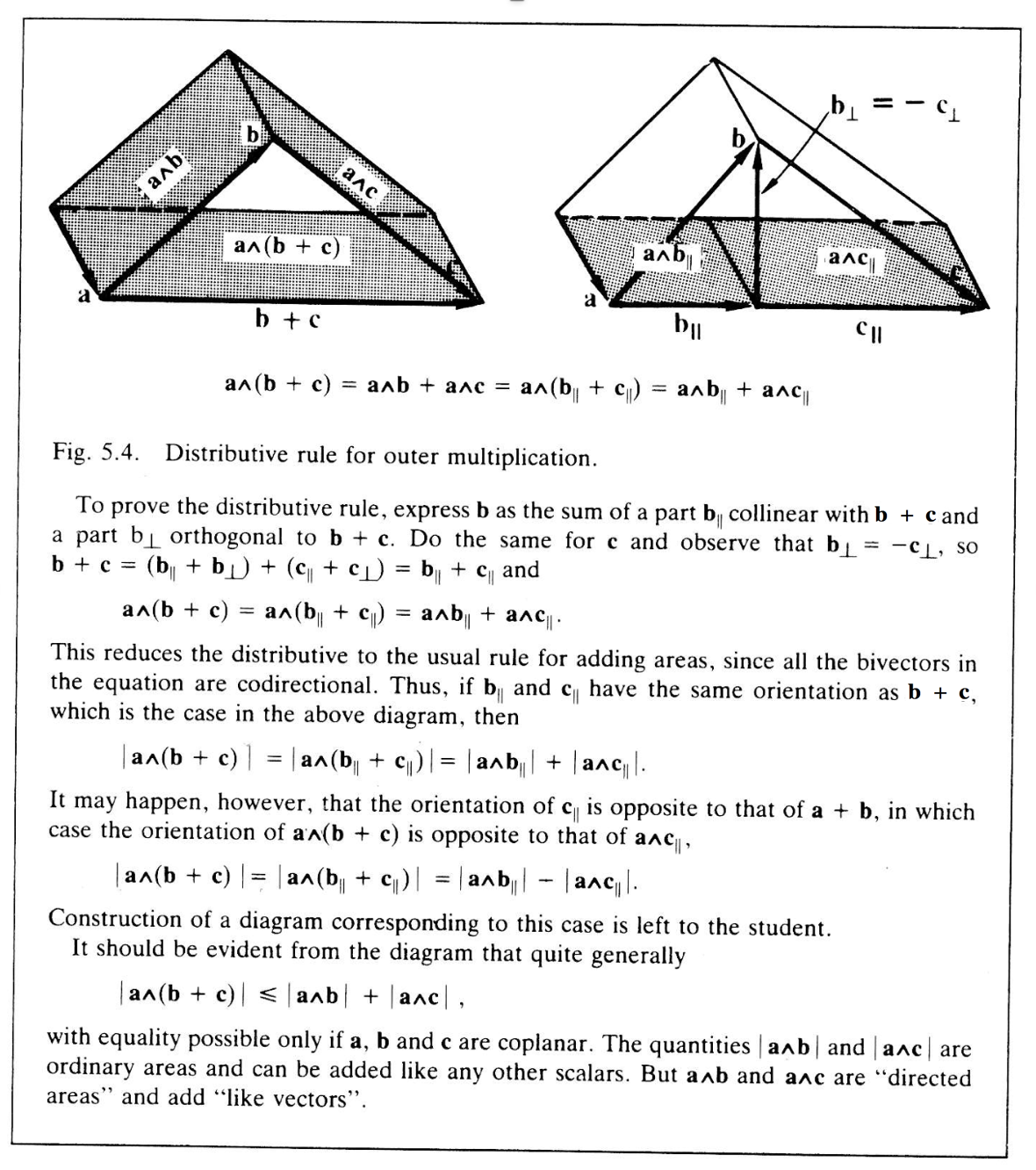
Fig. 5.4.

The corresponding geometrical construction is illustrated in Figure 5.4. Note that (5.11) relates addition of vectors on the left to addition of bivectors on the right. So the algebraic properties and the geometrical interpretation of bivector addition are completely determined by the properties and interpretation already accorded to vector addition. For example, the sum of two bivectors is a unique bivector, and again, bivector addition is associative. For bivectors with the same direction, it is easily seen that the distributive rule (5.11) reduces to the usual rule for adding areas.

Both the inner and outer products are measures of relative direction, but they complement one another. Relations which are difficult or impossible to obtain with one may be easy to obtain with the other. Whereas the equation \, \bold a \cdot \bold b = 0 \, provides a simple expression of “perpendicular”, \, \bold a \wedge \bold b = 0 \, provides a simple expression of “parallel”. To illustrate the point, reconsider the vector equation for a triangle, which was analyzed above with the help of the inner product. Take the outer product of \, \bold a + \bold b = \bold c \, successively with vectors \, \bold a, \bold b, \bold c , and use the rules (5.10) and (5.11) to obtain the three equations

\, \bold a \wedge \bold b = \bold a \wedge \bold c ,
\, \bold b \wedge \bold a = \bold b \wedge \bold c ,
\, \bold c \wedge \bold a + \bold c \wedge \bold b = 0 .

Only two of these equations are independent; the third, for instance, is the sum of the first two. It is convenient to write the first two equations on a single line, like so:

\, \bold a \wedge \bold c = \bold a \wedge \bold b = \bold c \wedge \bold b. \;\;\;\;\;\;\;\;\;\;\;\;\;\;\;\;\;\;\;\;\;\;\;\;\;\;\;\;\;\;\;\;\;\;\;\;\;\;\;\;\;\;\;\;\;\;\;\;\;\;\;\;\;\;\;\;\;\;\;\;\;\; (5.12)

Here are three different ways of expressing the same bivector as a product of vectors. This gives three different ways of expressing its magnitude:

\, | \, \bold a \wedge \bold c \, | = \ \, \bold a \wedge \bold b \, | = | \, \bold c \wedge \bold b \, |. \;\;\;\;\;\;\;\;\;\;\;\;\;\;\;\;\;\;\;\;\;\;\;\;\;\;\;\;\;\;\;\;\;\;\;\;\;\;\;\;\;\;\;\;\;\;\;\;\;\;\;\; (5.13)

Using (5.4) and the scalar labels for a triangle indicated in Figure 4.4, one gets, after dividing with \, a \, b \, c ,

\, \dfrac {\sin A} {a} = \dfrac {\sin B} {b} = \dfrac {\sin C} {c}. \;\;\;\;\;\;\;\;\;\;\;\;\;\;\;\;\;\;\;\;\;\;\;\;\;\;\;\;\;\;\;\;\;\;\;\;\;\;\;\;\;\;\;\;\;\;\;\;\;\;\;\;\;\;\;\;\;\;\;\, (5.14)

This formula is called the “law” of sines in trigonometry. We shall see in Chapter 2 that all the formulas of plane and spherical trigonometry can be easily derived and compactly expressed by using inner and outer products.

The theory of the outer product as described so far calls for an obvious generalization. Just as a plane segment is swept out by a moving line segment, a “space segment” is swept out by a moving plane segment. Thus, the points on an oriented parallelogram specified by a bivector \, \bold a \wedge \bold b \, moving a distance and direction specified by a vector \, \bold c \, sweep out an oriented parallelepiped (Figure 5.5), which may be characterized by a new kind of directed number \, \bold T \, called a trivector or 3-vector. The properties of \, \bold T \, are fixed by regarding it as equal to the outer product of the bivector \, \bold a \wedge \bold b \, with the vector \, \bold c . So write

\, (\bold a \wedge \bold b) \wedge \bold c = T \;\;\;\;\;\;\;\;\;\;\;\;\;\;\;\;\;\;\;\;\;\;\;\;\;\;\;\;\;\;\;\;\;\;\;\;\;\;\;\;\;\;\;\;\;\;\;\;\;\;\;\;\;\;\;\;\;\;\;\;\;\;\;\;\;\;\;\;\;\;\;\; (5.15)

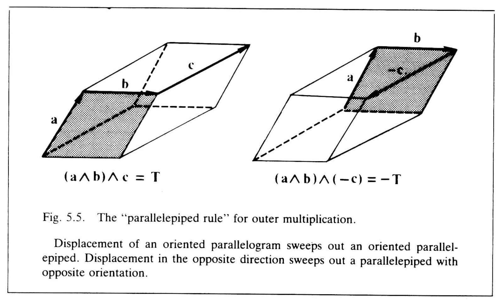
Fig. 5.5.

The study of trivectors leads to results quite analogous to those obtained above for bivectors, so the analysis need not be carried out in detail. But one new result obtains, namely, the conclusion that outer multiplication should obey the associative rule:

\, (\bold a \wedge \bold b) \wedge \bold c = \bold a \wedge (\bold b \wedge \bold c). \;\;\;\;\;\;\;\;\;\;\;\;\;\;\;\;\;\;\;\;\;\;\;\;\;\;\;\;\;\;\;\;\;\;\;\;\;\;\;\;\;\;\;\;\;\;\;\;\;\;\;\;\;\;\;\; (5.16)

The geometric meaning of associativity can be ascertained with the help of the following rule:

\, (\bold b \wedge \bold a) \wedge \bold c = ( - \bold a \wedge \bold b) \wedge \bold c) = - \bold T. \;\;\;\;\;\;\;\;\;\;\;\;\;\;\;\;\;\;\;\;\;\;\;\;\;\;\;\;\;\;\;\;\;\;\;\;\;\;\;\;\; (5.17)

This is an instance of the general rule that the orientation of a product is reversed by reversing the orientation of one of its factors. Repeated applications of (5.16) and (5.17) makes it possible to rearrange the vectors in a product to get

\, (\bold a \wedge \bold b) \wedge \bold c = (\bold b \wedge \bold c) \wedge \bold a = (\bold c \wedge \bold a) \wedge \bold b .

This says that the same oriented parallelepiped is obtained by sweeping \, "\bold a \wedge \bold b \, along \, \bold c" , \, "\bold b \wedge \bold c \, along \, \bold a" , or \, "\bold c \wedge \bold a \, along \, \bold b" . So the associative rule is needed to express the equivalence of different ways of “building up” a space element out of line segments.

Of course, if \, \bold c \, “lies in the plane of \, \bold a \wedge \bold b “, then “sweeping \, \bold a \wedge \bold b \, along \, \bold c ” does not produce a 3-dimensional object. Accordingly, write

\, (\bold a \wedge \bold b) \wedge \bold c = \bold a \wedge \bold b \wedge \bold c = 0. \;\;\;\;\;\;\;\;\;\;\;\;\;\;\;\;\;\;\;\;\;\;\;\;\;\;\;\;\;\;\;\;\;\;\;\;\;\;\;\;\;\;\;\;\;\;\;\;\;\;\; (5.18)

This equation produces a simple algebraic way of saying that 3 lines (with directions denoted by vectors \, \bold a, \, \bold b, \, \bold c ) lie in the same plane, just as Equation (5.9) provides a simple way of saying that 2 lines are parallel.

Like any other directed number, a 3 vector has magnitude, direction and orientation, and only these properties. The dimensionality of a 3-vector is expressed by the fact that it can be factored into an outer product of three vectors, though this can be done in an unlimited number of ways. The magnitude of \, \bold a \wedge \bold b \wedge \bold c \, is denoted by \, | \, \bold a \wedge \bold b \wedge \bold c \, | \, and is equal to the volume of the parallepiped determined by the vectors \, \bold a, \, \bold b \, and \, \bold c .

The orientation of a trivector depends on the order of its factors. The anticommutation rule together with the associative rule imply that the exchange of any pair of factors in a product reverses the orientation of the result. For instance, latex] \, \bold c \wedge \bold b \wedge \bold a = – \bold a \wedge \bold b \wedge \bold c [/latex]. Thus the idea of relative orientation is very easily expressed with the help of the outer product. Without such an algebraic apparatus the geometrical idea of orientation is quite difficult to express, and, not surprisingly, was only dimly understood before the invention of vectors and the outer product.

The essential aspects of outer multiplication and the generalized notions of number and direction it entails have now been set down. No fundamentally new insights into the relations between algebra and geometry are achieved by considering the outer product of four or more vectors. But it should be mentioned that if vectors are used to describe the 3-dimensional space of ordinary geometry, then displacement of the trivector \, \bold a \wedge \bold b \wedge \bold c \, in a direction specified by \, \bold d \, fails to sweep out a 4-dimensional space segment so write

\, (\bold a \wedge \bold b \wedge \bold c) \wedge \bold d = \bold a \wedge \bold b \wedge \bold c \wedge \bold d = 0. \;\;\;\;\;\;\;\;\;\;\;\;\;\;\;\;\;\;\;\;\;\;\;\;\;\;\;\;\;\;\;\;\;\;\;\;\;\; (5.19)

The parenthesis is unnecessary because of the associative rule (5.16). Equation (5.19) must hold for any four vectors \, \bold a, \, \bold b, \, \bold c, \bold d . This is a simple way of saying that space is 3-dimensional. Note the similarity in form and meaning of Equations (5.19), (5.18) and (5.9). It should be clear that (5.19) does not follow from any ideas or rules previously considered. By supposing that the outer product of four vectors is not zero, one is led to an algebraic description of spaces and geometries of four or more dimensions, but we already have what we need to describe the geometrical properties of physical space.

The outer product was invented by Hermann Grassmann, and, following a line of thought similar to the one above, he developed it into a complete mathematical theory before the middle of the nineteenth century. His theory has been accorded a prominent place in mathematics only in the last forty years, and it is hardly known at all to physicists.

Grassmann himself was the only one to use it during the first two decades after it was published. There are several reasons for this. The most important one arises from the fact that Grassmann’s understanding of the abstract nature of mathematics was far ahead of his time. He was the first person to arrive at the modern conception of algebra as a system of rules relating otherwise undefined entities. He realized that the nature of the outer product could be defined by specifying the rules it obeys, especially the distributive, associative, and anticommutative rules given above.

He rightly expounded this momentous insight in great detail. And he proved its significance by showing, for the first time, how abstract algebra can take us beyond the 3-dimensional space of experience to a conception of space with any number of dimensions.

Unfortunately, in his enthusiasm for abstract developments, Grassmann deemphasized the geometric origin and interpretation of his rules.. No doubt many potential readers would have appreciated the geometrical applications of Grassmann’s system, but most were simply confounded by the profusion of unfamiliar abstract ideas in Grassmann’s long books.

The seeds of Hermann Grassmann’s great invention were sown by his father Günther, who in 1824, when Hermann was 15, published these words in a book intended for elementary instruction:

“the rectangle itself is the true geometrical product, and the construction of it is really geometrical multiplication…. A rectangle is the geometric product of its base and height, and this product behaves in the same way as the arithmetic product.” (italics added)

The elder Grassmann elaborated his idea at some length and must have advocated it with considerable enthusiasm to his young son. As it stands, however, Günther’s idea is hardly more than a novel way of expressing the central idea of Book II of Euclid’s Elements. The Greeks made frequent use of the correspondence between the product of numbers and the constrtuction of a parallelogram from its base and height. For example, Euclid represented the distributive rule of algebra as addition of areas and proved it as a geometrical theorem.

This correspondence between arithmetic and geometry was rejected by Descartes and duly ignored by the mathematicians that followed him. However, as already explained, Descartes merely associated arithmetic multiplication with a different geometric construction. The old Greek idea lay dormant until it was reexpressed in strong arithmetic terms by Günther Grassmann. But the truly significant advance, from the idea of a geometrical product to its full algebraic expression by outer multiplication, was made by his son.

Hermann Grassmann completed the algebraic formulation of basic ideas on Greek geometry begun by Descartes. The Greek theory of ratio and proportion is now incorporated in the properties of scalars and scalar multiplication. The Greek idea of projection is incorporated in the inner product. And the Greek geometrical product is expressed by outer multiplication. The invention of a system of directed numbers to express Greek geometrical notions makes it possible, as Descartes had already said, to go far beyond the geometry of the Greeks. It also leads to a deeper appreciation of the Greek accomplishments.

Only in the light of Grassmann’s outer product is it possible to understand that the careful Greek distinction between number and magnitude has real geometrical significance. It corresponds roughly to the distinction between scalar and vector. Actually the Greek magnitudes added like scalars but multiplied like vectors, so multiplication of Greek magnitudes involves the notion of direction and dimension, and Euclid was quite right in distinguishing it from multiplication of “Greek numbers” (our scalars). Only in the work of Grassmann are the notions of direction, dimension, orientation and scalar magnitude fully disentangled. But his great accomplishment would have been impossible without the earlier vague distinction of the Greeks, and perhaps without its reformulation in quasi-arithmetic terms by his father.

1-6. Synthesis and Simplification

Grassmann was the first person to define multiplication simply by specifying a set of algebraic rules. By systematically surveying various possible rules, he discovered several other kinds of multiplication besides his inner and outer products. Nevertheless, he overlooked the most important possibility until late in his life, when he was unable to follow up on its implications. There is one fundamental kind of geometric product from which all other significant geometric products can be obtained. All the geometrical facts needed to discover such a product have been mentioned before.

It has already been noted that the inner and outer products seem to complement one another by describing independent geometrical relations. This circumstance deserves the most careful study. The simplest approach is to entertain the possibility of introducing a new kind of product \, \bold a \, \bold b \, by the equation

\, \bold a \, \bold b \stackrel {\mathrm{def}}{=} \bold a \cdot \bold b + \bold a \wedge \bold b. \;\;\;\;\;\;\;\;\;\;\;\;\;\;\;\;\;\;\;\;\;\;\;\;\;\;\;\;\;\;\;\;\;\;\;\;\;\;\;\;\;\;\;\;\;\;\;\;\;\;\;\;\;\;\;\;\;\;\;\;\;\;\;\;\;\;\;\;\;\; (6.1)

Here the scalar \, \bold a \cdot \bold b \, has been added to the bivector \, \bold a \wedge \bold b . At first sight it may seem absurd to add two different numbers with different grades. That may have delayed Grassmann from considering it. For centuries the notion that you can only add “like things” has been relentlessly impressed on the mind of every schoolboy. It is a kind of mathematical taboo – its real justification unknown or forgotten. It is supposedly obvious that you cannot add apples and oranges or feet and square feet. On the contrary, it is only obvious that addition of apples and oranges is not usually a practical thing to do – unless you are making a salad.

Absurdity disappears when it is realized that (6.1) can be justified in the abstract “Grassmannian” fashion which has become standard mathematical procedure today. All that mathematics really requires is that the indicated relations and operations be well defined and consistently employed. The mathematical meaning of adding scalars and bivectors is determined by verifying that such addition satisfy the usual commutative and associative rules.Use of the equality sign in (6.1) is justified by verifying that this geometric product obeys the same rules as those governing equality in ordinary scalar algebra. With this understood, it now can be shown that the properties of the new product are almost completely determined by the obvious requirement that they be consistent with the properties already accorded to the inner and outer products.

The commutative rule \, \bold b \cdot \bold a = \bold a \cdot \bold b \, together with the anticommutative rule
\, \bold b \wedge \bold a = -\bold a \wedge \bold b \, imply a relation between \, \bold a \, \bold b \, and \, \bold b \, \bold a . Thus

\, \bold b \, \bold a = \bold b \cdot \bold a + \bold b \wedge \bold a = \bold a \cdot \bold b - \bold a \wedge \bold b. \;\;\;\;\;\;\;\;\;\;\;\;\;\;\;\;\;\;\;\;\;\;\;\;\;\;\;\;\;\;\;\;\;\;\;\;\;\;\;\;\;\;\;\;\; (6.2)

Comparison of (6.1) and (6.2) shows that, in general, \, \bold a \, \bold b \, is not equal to \, \bold b \, \bold a \, because, though their scalar parts are equal, their bivector parts are not.

However, if \, \bold a \wedge \bold b = 0 , then

\, \bold a \, \bold b = \bold a \cdot \bold b = \bold b \, \bold a. \;\;\;\;\;\;\;\;\;\;\;\;\;\;\;\;\;\;\;\;\;\;\;\;\;\;\;\;\;\;\;\;\;\;\;\;\;\;\;\;\;\;\;\;\;\;\;\;\;\;\;\;\;\;\;\;\;\;\;\;\;\;\;\;\;\;\;\;\;\;\;\; (6.3)

And if \, \bold a \cdot \bold b = 0 , then

\, \bold a \, \bold b = \bold a \wedge \bold b = - \bold b \wedge \bold a = - \bold b \,\bold a. \;\;\;\;\;\;\;\;\;\;\;\;\;\;\;\;\;\;\;\;\;\;\;\;\;\;\;\;\;\;\;\;\;\;\;\;\;\;\;\;\;\;\;\;\;\;\;\;\;\;\;\; (6.4)

It should not escape notice that to get (6.3) and (6.4) from (6.1) the usual “additive property of zero” is needed, and no distinction between a scalar zero and a bivector zero is called for.

The product \, \bold a \, \bold b \, inherits a geometrical interpretation from the interpretations already accorded to the inner and outer products. It is an algebraic measure of the relative direction of the vectors \, \bold a \, and \, \bold b . Thus, from (6.3) and (6.4) it should be clear that vectors are collinear if and only if their product is commutative and they are orthogonal if and only if their product is anticommutative. But more properties of the product are required to understand its significance when the relative direction of the two vectors is somewhere between the extremes of collinearity and orthogonality.

To give due recognition to its geometric significance, \, \bold a \, \bold b \, will henceforth be called the geometric product of vectors \, \bold a \, and \, \bold b .

From the distributive rules (4.4) and (5.11) for inner and outer products, it follows that the geometric product must obey the left and right distributive rules

\, \bold a \, ( \bold b + \bold c ) = \bold a \, \bold b + \bold a \, \bold c. \;\;\;\;\;\;\;\;\;\;\;\;\;\;\;\;\;\;\;\;\;\;\;\;\;\;\;\;\;\;\;\;\;\;\;\;\;\;\;\;\;\;\;\;\;\;\;\;\;\;\;\;\;\;\;\;\;\;\;\;\;\;\;\;\; (6.5)

\, ( \bold b + \bold c ) \, \bold a = \bold b \, \bold a + \bold c \, \bold a. \;\;\;\;\;\;\;\;\;\;\;\;\;\;\;\;\;\;\;\;\;\;\;\;\;\;\;\;\;\;\;\;\;\;\;\;\;\;\;\;\;\;\;\;\;\;\;\;\;\;\;\;\;\;\;\;\;\;\;\;\;\;\;\;\; (6.6)

Equation (6.5) can be derived from (6.1) by the following steps

\, \bold a \, ( \bold b + \bold c ) = \bold a \cdot ( \bold b + \bold c) + \bold a \, ( \bold b \wedge \bold c ) = = \, ( \bold a \cdot \bold b + \bold a \cdot \bold c ) + ( \bold a \wedge \bold b + \bold a \wedge \bold c ) = = \, ( \bold a \cdot \bold b + \bold a \wedge \bold b ) + ( \bold a \cdot \bold c + \bold a \wedge \bold c ) =

= \, \bold a \, \bold b + \bold a \, \bold c .

Note that the usual properties of equality and the commutative and associative rules of addition have been employed. Equation (6.6) can be derived from (6.2) in the same way. The distributive rules (6.5) and (6.6) are independent of one another, because multiplication is not commutative. To derive them, the distributive rules for both the inner and outer products were needed.

The relation of scalar multiplication to the geometric product is described by the equations

\, \lambda \, \bold a \, \bold b = ( \lambda \, \bold a ) \, \bold b = \bold a \, ( \lambda \, \bold b ). \;\;\;\;\;\;\;\;\;\;\;\;\;\;\;\;\;\;\;\;\;\;\;\;\;\;\;\;\;\;\;\;\;\;\;\;\;\;\;\;\;\;\;\;\;\;\;\;\;\;\;\;\;\;\;\;\;\;\; (6.7)

This is easily derived from (4.3) and (5.8) with the help of the definition (6.1). It says that the scalar and vector multiplication are mutually commutative and associative. If the commutative rule is separated from the associative rule, it takes the simple form

\, \lambda \, \bold a = \bold a \lambda. \;\;\;\;\;\;\;\;\;\;\;\;\;\;\;\;\;\;\;\;\;\;\;\;\;\;\;\;\;\;\;\;\;\;\;\;\;\;\;\;\;\;\;\;\;\;\;\;\;\;\;\;\;\;\;\;\;\;\;\;\;\;\;\;\;\;\;\;\;\;\;\;\;\;\;\;\;\;\;\;\;\;\;\, (6.8)

Now observe that by taking the sum and difference of equations (6.1) and (6.2), one gets

\, \bold a \cdot \bold b = \frac{1}{2} ( \bold a \, \bold b + \bold b \, \bold a), \;\;\;\;\;\;\;\;\;\;\;\;\;\;\;\;\;\;\;\;\;\;\;\;\;\;\;\;\;\;\;\;\;\;\;\;\;\;\;\;\;\;\;\;\;\;\;\;\;\;\;\;\;\;\;\;\;\;\;\;\;\;\;\;\;\; (6.9)

and

\, \bold a \wedge \bold b = \frac{1}{2} ( \bold a \, \bold b - \bold b \, \bold a). \;\;\;\;\;\;\;\;\;\;\;\;\;\;\;\;\;\;\;\;\;\;\;\;\;\;\;\;\;\;\;\;\;\;\;\;\;\;\;\;\;\;\;\;\;\;\;\;\;\;\;\;\;\;\;\;\;\;\;\;\;\;\;\; (6.10)

This points the way to a great simplification. Instead of regarding (6.1) as a definition of \, \bold a \,\bold b , consider \, \bold a \, \bold b \, as fundamental and regard (6.9) and (6.10) as definitions of \, \bold a \cdot \bold b \, and \, \bold a \wedge \bold b . This reduces two kinds of vector multiplication to one. It is curious, then, to note that by (6.7) the commutativity of the inner product arises from the commutativity of addition, and by (6.10) the anticommutativity of the outer product arises from the anticommutativity of subtraction.

The algebraic properties of the geometric product of two vectors have already been ascertained. It should be evident that the corresponding properties of the inner and outer products can be derived from the definitions (6.9) and (6.10) simply by reversing the arguments already given.

The next task is to examine the geometric product of three vectors \, \bold a, \bold b, \bold c . It is certainly desirable that this product satisfy the associative rule

\, \bold a \, (\bold b \, \bold c) = (\bold a \, \bold b) \, \bold c, \;\;\;\;\;\;\;\;\;\;\;\;\;\;\;\;\;\;\;\;\;\;\;\;\;\;\;\;\;\;\;\;\;\;\;\;\;\;\;\;\;\;\;\;\;\;\;\;\;\;\;\;\;\;\;\;\;\;\;\;\;\;\;\;\;\;\;\;\;\;\;\; (6.11)

for that greatly simplifies algebraic manipulations. But it must be shown that this rule reproduces established properties of the inner and outer products. This can be done by examining the geometric product of a vector with a bivector.

The product \, \bold a \,\bold B \, of a vector \, \bold a \, with a bivector \, \bold B \, can be expressed as a sum of “symmetric” and “antisymmetric” parts in the following way

\, \bold a \,\bold B = \frac{1}{2} (\bold a \, \bold B + \bold a \, \bold B) + \frac{1}{2} (\bold B \, \bold a - \bold B \, \bold a) =

\;\;\;\;\;\;\; = \frac{1}{2} (\bold a \, \bold B - \bold B \, \bold a) + \frac{1}{2} (\bold a \,\bold B + \bold B \, \bold a) .

Anticipating results to be obtained, introduce the notations

\, \bold a \cdot \bold B = \frac{1}{2} (\bold a \, \bold B - \bold B \, \bold a) = - \bold B \cdot \bold a, \;\;\;\;\;\;\;\;\;\;\;\;\;\;\;\;\;\;\;\;\;\;\;\;\;\;\;\;\;\;\;\;\;\;\;\;\;\;\;\;\;\;\;\;\;\;\;\; (6.12)

\, \bold a \wedge \bold B = \frac{1}{2} (\bold a \, \bold B + \bold B \, \bold a) = \bold B \wedge \bold a, \;\;\;\;\;\;\;\;\;\;\;\;\;\;\;\;\;\;\;\;\;\;\;\;\;\;\;\;\;\;\;\;\;\;\;\;\;\;\;\;\;\;\;\;\;\;\;\; (6.13)

So

\, \bold a \,\bold B = \bold a \cdot \bold B + \bold a \wedge \bold B. \;\;\;\;\;\;\;\;\;\;\;\;\;\;\;\;\;\;\;\;\;\;\;\;\;\;\;\;\;\;\;\;\;\;\;\;\;\;\;\;\;\;\;\;\;\;\;\;\;\;\;\;\;\;\;\;\;\;\;\;\;\;\;\;\; (6.14)

As the notation indicates, \, \bold a \wedge \bold B \, is to be regarded as identical to the outer product of a vector and a bivector which has already been introduced for geometric reasons. The quantity \, \bold a \cdot \bold B \, is something new: as the notation suggests, it is to be regarded as a generalization of the inner product of vectors.

Note that (6.13) differs from (6.10) by a sign, because (6.13) has a bivector where (6.19 has a vector. The sign in (6.13) is justified by showing that (6.13) yields the properties already ascribed to the outer product. To this end, it is sufficient to show that (6.13) implies the associative rule \, (\bold a \wedge \bold b) \wedge \bold c = \bold a \wedge (\bold b \wedge \bold c) . Of course the properties of the geometric product, including the associative rule (6.11) must be freely used in the proof.

[…]

Now to understand the significance of \, \bold a \cdot \bold B , let \, \bold B = \bold b \wedge \bold c . Use the definitions as before to eliminate the dot and the wedge:

\, \bold a \cdot (\bold b \wedge \bold c) = \frac{1}{2} \, [ \, \bold a \, \frac{1}{2} \, ( \bold b \, \bold c - \bold c \, \bold b) - \frac{1}{2} \, ( \bold b \, \bold c - \bold c \, \bold b) \, \bold a \, ] =

\,\;\;\;\;\;\;\;\;\;\;\;\;\;\;\;\;\, = \frac{1}{4} \, [ \, \bold a \, \bold b \, \bold c - \bold a \, \bold c \, \bold b - \bold b \, \bold c \, \bold a + \bold c \, \bold b \, \bold a \, ] .

To this, add

\, 0 = \frac{1}{4} \, [ \, \bold b \, \bold a \, \bold c - \bold c \, \bold a \, \bold b - \bold b \, \bold a \, \bold c + \bold c \, \bold a \, \bold b \, ] ,

and collect terms to get

\, \bold a \cdot (\bold b \wedge \bold c) = \, = \frac{1}{4} \, [ \, (\bold a \, \bold b + \bold b \, \bold a) \, \bold c - (\bold a \, \bold c + \bold c \, \bold a) \, \bold b - \bold b \, (\bold c \, \bold a + \bold a \, \bold c) + \bold c \, (\bold b \, \bold a + \bold a \, \bold b) \, ] = \, = \frac{1}{4} \, [ \, 2 \, (\bold a \cdot \bold b) \, \bold c - 2 \, (\bold a \cdot \bold c) \, \bold b - \bold b \, 2 \, (\bold a \cdot \bold c) + \bold c \, 2 \, (\bold b \cdot \bold a) \, ] =

\, = (\bold a \cdot \bold b) \, \bold c - (\bold a \cdot \bold c) \, \bold b .

Thus

\, \bold a \cdot (\bold b \wedge \bold c) = (\bold a \cdot \bold b) \, \bold c - (\bold a \cdot \bold c) \, \bold b. \;\;\;\;\;\;\;\;\;\;\;\;\;\;\;\;\;\;\;\;\;\;\;\;\;\;\;\;\;\;\;\;\;\;\;\;\;\;\;\;\;\;\;\;\;\;\; (6.15)

This shows that inner multiplication of a vector with a bivector results in a vector. So Equation (6.14) expresses the fact that the geometric product \, \bold a \, \bold B \, of a vector and a bivector results in the sum of a vector \, \bold a \cdot \bold B \, and a trivector \, \bold a \wedge \bold B .

The similarity between (6.1) and (6.14) should be noted. They illustrate the general rule that outer multiplication by a vector “raises the dimension” of any directed number by one, whereas inner multiplication “lowers” it by one. Clearly, the generalized inner and outer products provide an algebraic vehicle for expressing geometric notions about “decreasing or increasing the dimension of space”.

1-7. Axioms for Geometric Algebra

Let us examine now what we have learned about building a geometric algebra. To begin with, the algebra should include the graded elements 0-vector, 1-vector, 2-vector and 3-vector to represent the directional properties of points, lines, planes and space. We introduced three different kinds of multiplication, the scalar, inner and outer products, to express relations among the elements. But we saw that inner and outer products can be reduced to a single geometric product if we allow elements of different grade (or dimension) to be added. For this reason, we conclude that the algebra should include elements of “mixed grade”, such as

\, A = A_0 + {\bold A}_1 + {\bold A}_2 + {\bold A}_3. \;\;\;\;\;\;\;\;\;\;\;\;\;\;\;\;\;\;\;\;\;\;\;\;\;\;\;\;\;\;\;\;\;\;\;\;\;\;\;\;\;\;\;\;\;\;\;\;\;\;\;\;\;\;\;\;\;\;\, (7.1)

Before continuing, a note about nomenclature is in order. The term “dimension” has two distinct but closely related mathematical meanings. To separate them we will henceforth use the term “grade” exclusively to mean “dimension” in the sense that we have used the term up to this point. We have preferred the term “dimension” in our introductory discussion, because it is likely to have familiar and helpful connotations for the reader. However, now we aim to improve the precision of our language with an axiomatic formulation of the basic concepts. the alternative meaning for “dimension” will be explained in Section 2.2, where for \, k = 0, 1, 2, 3 , \, {A}_k is an element of grade \, k called the \, k -vector part of \, A . Thus (7.1) presents \, A \, as the sum of a scalar \, A_0 \, , a vector \, {\bold A}_1 \, , a bivector \, {\bold A}_2 \, and a trivector \, {\bold A}_3 . We refer to \, A \, as a multivector, a (directed) number or a quantity.

Any element of the geometric algebra can be called a multivector, because it can be represented in the form (7.1). For example, a vector \, \bold a \, can be expressed trivially in the form (7.1) by writing \, A = {\bold A}_1 = \bold a \, , A_0 = {\bold A}_2 = {\bold A}_3 = 0 \, and using the property \, \bold a + 0 = \bold a . Note that the \, k -vectors which are not scalars are denoted by symbols in boldface type. Such \, k -vectors are sometimes called \, k –blades or simply, blades to emphasize the fact that, in contrast to \, 0 -vectors (scalars), they have “directional properties”.

Now another simplification becomes possible. It will be noted that the geometric product of vectors, which we have just considered has, except for commutivity, the same algebraic properties as scalar multiplication of vectors and bivectors. In particular, both products are associative and distributive with respect to addition. Rather than regard them as two different kinds of multiplication, we can regard them as instances of a single geometric product among different kinds of multivector. Thus, scalar multiplication is the geometric product of any multivector by a special kind of multivector called a scalar. The special geometric nature of the scalars is expressed algebraically by the fact that they commute with every other multivector.

Thus we define addition and multiplication of multivectors by the following familiar rules: For multivectors \, A, B, C, \cdots \, , addition is commutative,

\, A + B = B + A; \;\;\;\;\;\;\;\;\;\;\;\;\;\;\;\;\;\;\;\;\;\;\;\;\;\;\;\;\;\;\;\;\;\;\;\;\;\;\;\;\;\;\;\;\;\;\;\;\;\;\;\;\;\;\;\;\;\;\;\;\;\;\;\;\;\;\;\;\;\;\;\, (7.2)

addition and multiplication are associative,

\, (A + B) + C = A + (B + C), \;\;\;\;\;\;\;\;\;\;\;\;\;\;\;\;\;\;\;\;\;\;\;\;\;\;\;\;\;\;\;\;\;\;\;\;\;\;\;\;\;\;\;\;\;\;\;\;\;\;\;\, (7.3)

\, (A B) \, C = A \, (B \, C); \;\;\;\;\;\;\;\;\;\;\;\;\;\;\;\;\;\;\;\;\;\;\;\;\;\;\;\;\;\;\;\;\;\;\;\;\;\;\;\;\;\;\;\;\;\;\;\;\;\;\;\;\;\;\;\;\;\;\;\;\;\;\;\;\;\;\; (7.4)

multiplication is distributive with respect to addition,

\, A \, (B + C) = A \, B + A \, C, \;\;\;\;\;\;\;\;\;\;\;\;\;\;\;\;\;\;\;\;\;\;\;\;\;\;\;\;\;\;\;\;\;\;\;\;\;\;\;\;\;\;\;\;\;\;\;\;\;\;\;\;\;\;\;\;\;\; (7.5)

\, (B + C) \, A = B \, A + C \, A. \;\;\;\;\;\;\;\;\;\;\;\;\;\;\;\;\;\;\;\;\;\;\;\;\;\;\;\;\;\;\;\;\;\;\;\;\;\;\;\;\;\;\;\;\;\;\;\;\;\;\;\;\;\;\;\;\;\; (7.6)

There exist unique multivectors \, 0 \, and \, 1 \, such that

\, A + 0 = A, \;\;\;\;\;\;\;\;\;\;\;\;\;\;\;\;\;\;\;\;\;\;\;\;\;\;\;\;\;\;\;\;\;\;\;\;\;\;\;\;\;\;\;\;\;\;\;\;\;\;\;\;\;\;\;\;\;\;\;\;\;\;\;\;\;\;\;\;\;\;\;\;\;\;\;\;\;\;\; (7.7)

\, 1 \, A = A. \;\;\;\;\;\;\;\;\;\;\;\;\;\;\;\;\;\;\;\;\;\;\;\;\;\;\;\;\;\;\;\;\;\;\;\;\;\;\;\;\;\;\;\;\;\;\;\;\;\;\;\;\;\;\;\;\;\;\;\;\;\;\;\;\;\;\;\;\;\;\;\;\;\;\;\;\;\;\;\;\;\;\, (7.8)

Every multivector \, A \, has a unique additive inverse \, - A , that is

\, A + (- A) = 0. \;\;\;\;\;\;\;\;\;\;\;\;\;\;\;\;\;\;\;\;\;\;\;\;\;\;\;\;\;\;\;\;\;\;\;\;\;\;\;\;\;\;\;\;\;\;\;\;\;\;\;\;\;\;\;\;\;\;\;\;\;\;\;\;\;\;\;\;\;\;\;\;\; (7.9)

Of course, the whole algebra is assumed to be algebraically closed, that is, the sum or product of any two multivectors is itself a unique multivector.

It is hardly necessary to discuss the significance of the above axioms, since they are familiar from the elementary algebra of scalars. They can be used to manipulate multivectors in exactly the same way that numbers are manipulated in arithmetic. For example, axiom (7.9) is used to define subtraction of arbitrary multivectors in the same way that subtraction of vectors was defined by Equation (3.10).

To complete our system of axioms for geometric algebra, we need some axioms that characterize the various kinds of \, k -vectors. First of all, we assume that the set of all scalars in the algebra can be identified with the real numbers, and we express the commutivity of scalar multiplication by the axiom

\, \lambda \, A = A \, \lambda \;\;\;\;\;\;\;\;\;\;\;\;\;\;\;\;\;\;\;\;\;\;\;\;\;\;\;\;\;\;\;\;\;\;\;\;\;\;\;\;\;\;\;\;\;\;\;\;\;\;\;\;\;\;\;\;\;\;\;\;\;\;\;\;\;\;\;\;\;\;\;\;\;\;\;\;\;\;\;\;\;\; (7.10)

for every scalar \, \lambda \, and multivector \, A . Vectors are characterized by the following axiom. The “square” of any nonzero vector \, \bold a \, is a unique positive number \, | \,\bold a \, |^2 , that is,

\, {\bold a}^2 = | \,\bold a \, |^2 > 0. \;\;\;\;\;\;\;\;\;\;\;\;\;\;\;\;\;\;\;\;\;\;\;\;\;\;\;\;\;\;\;\;\;\;\;\;\;\;\;\;\;\;\;\;\;\;\;\;\;\;\;\;\;\;\;\;\;\;\;\;\;\;\;\;\;\;\;\;\;\;\;\;\;\;\; (7.11)

We characterize \, k -vectors of higher grade by relating them to vectors. It will be most convenient to do that after we introduce a couple of definitions.

For a vector \, \bold a \, and any \, k -blade \, {\bold A}_k we define the inner product by

\, \bold a \cdot {\bold A}_k = \frac{1}{2} \, ( \bold a {\bold A}_k - (-1)^k \, {\bold A}_k \, \bold a ), \, \;\;\;\;\;\;\;\;\;\;\;\;\;\;\;\;\;\;\;\;\;\;\;\;\;\;\;\;\;\;\;\;\;\;\;\;\;\;\;\;\;\;\;\;\;\;\, (7.12a)

and the outer product by

\, \bold a \wedge {\bold A}_k = \frac{1}{2} \, ( \bold a {\bold A}_k + (-1)^k \, {\bold A}_k \, \bold a ). \, \;\;\;\;\;\;\;\;\;\;\;\;\;\;\;\;\;\;\;\;\;\;\;\;\;\;\;\;\;\;\;\;\;\;\;\;\;\;\;\;\;\;\;\;\; (7.12b)

Adding these equations, we get

\, \bold a \, {\bold A}_k = \bold a \cdot {\bold A}_k + \bold a \wedge {\bold A}_k. \;\;\;\;\;\;\;\;\;\;\;\;\;\;\;\;\;\;\;\;\;\;\;\;\;\;\;\;\;\;\;\;\;\;\;\;\;\;\;\;\;\;\;\;\;\;\;\;\;\;\;\;\;\;\;\;\;\; (7.12c)

Note that (7.12a) includes (6.9) and (6.12) as special cases, while (7.12b) includes (6.10) and (6.13), and (7.12c) includes (6.1) and (6.14).

Using the definitions (7.12a) and (7.12b), we adopt the following propositions as axioms:

\, \bold a \cdot {\bold A}_k \, is a \, (k-1) -vector \,\;\;\;\;\;\;\;\;\;\;\;\;\;\;\;\;\;\;\;\;\;\;\;\;\;\;\;\;\;\;\;\;\;\;\;\;\;\;\;\;\;\;\;\;\;\;\;\;\;\;\;\;\;\;\;\;\;\; (7.13a)

\, \bold a \wedge {\bold A}_k \, is a \, (k+1) -vector. \,\;\;\;\;\;\;\;\;\;\;\;\;\;\;\;\;\;\;\;\;\;\;\;\;\;\;\;\;\;\;\;\;\;\;\;\;\;\;\;\;\;\;\;\;\;\;\;\;\;\;\;\;\;\;\;\; (7.13b)

Thus, the inner product lowers the grade of a \, k -vector, while the outer product raises the grade. According to (7.1), however, all \, k -vectors with grade \, k ≥ 4 \, must vanish. To assure this we need one more axiom: For every vector \, \bold a \, and \, 3 -vector \, {\bold A}_3 \, ,

\, \bold a \wedge {\bold A}_3 = 0. \;\;\;\;\;\;\;\;\;\;\;\;\;\;\;\;\;\;\;\;\;\;\;\;\;\;\;\;\;\;\;\;\;\;\;\;\;\;\;\;\;\;\;\;\;\;\;\;\;\;\;\;\;\;\;\;\;\;\;\;\;\;\;\;\;\;\;\;\;\;\;\;\;\;\;\;\, (7.14a)

By virtue of the definition (7.12b), this can alternatively be written

\, \bold a \, {\bold A}_3 = {\bold A}_3 \, \bold a. \;\;\;\;\;\;\;\;\;\;\;\;\;\;\;\;\;\;\;\;\;\;\;\;\;\;\;\;\;\;\;\;\;\;\;\;\;\;\;\;\;\;\;\;\;\;\;\;\;\;\;\;\;\;\;\;\;\;\;\;\;\;\;\;\;\;\;\;\;\;\;\;\;\;\, (7.14b)

In other words, vectors always commute with trivectors.

Finally, to assure that the whole algebraic system is not vacuous, we must assume that nonzero multivectors with all grades \, k ≤ 3 \, actually exist.

This completes our formulation of the axioms for geometric algebra. We have neglected some logical fine points (e.g., Exercise 7.1), but our axioms suffice to show exactly how geometric algebra generalizes the familiar algebra of scalars. We have chosen a notation for geometric algebra that is as similar as possible to the notation for scalar algebra. This is a point of great importance, for it facilitates the transfer of skills in manipulations with scalar algebra to manipulations with geometric algebra.

Axioms (7.2) to (7.9) implicitly define the operations of addition, subtraction and multiplication. Except for the absence of a general commutative law for multiplication, they are identical to the axioms for scalar algebra. Therefore, multivectors can be equated, added, subtracted and multiplied in exactly the same way as scalar quantities, provided one does not reorder multiplicative factors which do not commute. Division by multivectors can be defined in terms of multiplication, just as in scalar algebra. But we need to pay special attention to notation on account of noncommutativity, so let us consider the matter explicitely.

In geometric algebra, as in elementary algebra, the solution of equations is greatly facilitated by the possibility of division. We can divide by a multivector \, A \, if it has a multiplicative inverse. The inverse of \, A \, , if it exists, is denoted by \, A^{-1} or \, 1/A \, and defined by the equation

\, A^{-1} \, A = 1. \;\;\;\;\;\;\;\;\;\;\;\;\;\;\;\;\;\;\;\;\;\;\;\;\;\;\;\;\;\;\;\;\;\;\;\;\;\;\;\;\;\;\;\;\;\;\;\;\;\;\;\;\;\;\;\;\;\;\;\;\;\;\;\;\;\;\;\;\;\;\;\;\;\;\;\;\;\;\; (7.15)

We can divide any multivector \, B \, by \, A \, in two ways, by multiplying it by \, A^{-1} on the left,

\, A^{-1} \, B = \dfrac{ 1 }{ A } \, B \, ,

or on the right,

\, B \, A^{-1} = B \, \dfrac{ 1 }{ A } = B / A .

Obviously, the “left division” is not equivalent to the “right division” unless \, B \, commutes with \, A^{-1} , in which case the division can be denoted unambiguously by

\, \dfrac{ B }{ A } .

Every nonzero vector \, \bold a \, has a multiplicative inverse. To determine the inverse of \, \bold a , we multiply the equation \, {\bold a}^{-1} \bold a = 1 , on the right by \, \bold a \, and divide by the scalar \, {\bold a}^2 = | \, \bold a \, |^2 \, ; thus

\, {\bold a}^{-1} = \dfrac{\bold a }{ | \, \bold a \, |^2 }. \;\;\;\;\;\;\;\;\;\;\;\;\;\;\;\;\;\;\;\;\;\;\;\;\;\;\;\;\;\;\;\;\;\;\;\;\;\;\;\;\;\;\;\;\;\;\;\;\;\;\;\;\;\;\;\;\;\;\;\;\;\;\;\;\;\;\;\;\;\;\;\;\;\;\;\;\, (7.16)

With due regard for the order of factors, many tricks of elementary algebra, such as “rationalizing the denominator”, are equally useful in geometric algebra. It should be noted, however, that some multivectors do not have multiplicative inverses (see Exercise 7.2), so it is impossible to divide by them.

/////// End of quote from Hestenes