This page is a sub-page of our page on Calculus of Several Real Variables.
///////
Related KMR pages:
• Affine Geometry
• Complex Derivative
• Differentiation and Affine Approximation (in one real variable)
• The Chain Rule (in one real variable)
• The Chain Rule (in several real variables)
• Big-Ordo and Little-ordo notation
///////
Other related sources of information:
• The right way to think about derivatives and integrals
• Definition of the derivative as the linear part of the affine approximation
• Little-o notation
• The Cauchy-Riemann equations
• All pythagorean triples visualized through squaring of the gaussian integers.
• Logarithmic differentiation
• Affine geometry
• Affine Transformation
• o-notations, affine approximations and chain rule
• Courant, R., (1966, 1934): Differential and Integral Calculus, Vol. I (one real variable)
• Courant, R., (1964, 1936): Differential and Integral Calculus, Vol. II (several real variables)
• Snapper E. and Troyer, R. J., (1971): Metric Affine Geometry, Dover, 1989.
///////
The interactive simulations on this page can be navigated with the Free Viewer
of the Graphing Calculator.
///////
Anchors into the text below:
• The concept of differentiability
• Functions of several real variables
• The differential of a function
• Affine Maps
• Affine approximation of differentiable functions
• Forward and backward combinations of affine approximations
• Affine approximation from 1D to 1D
• Affine approximation from 2D to 1D
• Affine approximation from 2D to 2D
• Affine approximation from 3D to 3D
///////
Representation: \, [ \, p_{resentant} \, ]_{B_{ackground}} \, = \, \left< \, r_{epresentant} \, \right>_{B_{ackground}}
\, = \, [ \, D_{erivative} \, ]_{ \{ f : \, \mathbb{R} \to \mathbb{R} \} } \, = <br>
\, = \, \left< \, f'(x)_{\textcolor{blue}{p}} \, \stackrel {\mathrm{def}}{=} \, \lim\limits_{\textcolor{red}{\Delta x} \to 0} \dfrac {\textcolor{red}{\Delta f}} {\textcolor{red}{\Delta x}} \, \stackrel {\mathrm{def}}{=} \, \lim\limits_{\textcolor{red}{\Delta x} \to 0} \dfrac{f(\textcolor{blue}{p} + \textcolor{red}{\Delta x}) - f(\textcolor{blue}{p})} { \textcolor{red}{\Delta x} } \, \right>_{ \{ f : \, \mathbb{R} \to \mathbb{R} \} }\, [ \, A_{ffine}A_{pproximation} \, ]_{ \{ f : \, {\mathbb{R}}^n \to {\mathbb{R}}^m \} } \, = <br>
\, = \left< \, f_{\textcolor{blue}{p}}(x) \, \stackrel{\text{def}}{=} \, f_{\textcolor{blue}{p}}(\textcolor{blue}{p} + \textcolor{red}{\Delta x}) \, \stackrel{\text{def}}{=} \, f(\textcolor{blue}{p}) + f'(x)_{\textcolor{blue}{p}} \, \textcolor{red}{\Delta x} \, \right>_{ \{ f : \, {\mathbb{R}}^n \to {\mathbb{R}}^m \} } \,\, = \, [ \, The \, D_{erivative} \, of \, f(x) \, at the point \, x = \textcolor{blue}{p} \,\, ]_{ \{ f : \, {\mathbb{R}}^n \to {\mathbb{R}}^m \} } \, =
= \, < f'(x)_{\textcolor{blue}{p}} >_{ \{ f : \, {\mathbb{R}}^n \to {\mathbb{R}}^m \} } \, = <br>
= \, < The linear part of the affine approx. \, f_{\textcolor{blue}{p}}(x) \, of the function \, f(x) \, >_{ \{ f : \, {\mathbb{R}}^n \to {\mathbb{R}}^m \} } \;
///////
/////// Quoting (Courant, Vol. II, p.59):
4. THE TOTAL DIFFERENTIAL OF A FUNCTION AND ITS GEOMETRICAL MEANING
1. The concept of differentiability.
In the case of functions of one variable the existence of a derivative is intimately connected with the possibility of approximating the function \, \eta = f(\xi) \, in the neighborhood of the point \, x \, by means of a linear function \, \eta = \phi(\xi) . This linear function is defined by the equation
\, \phi(\xi) = f(x) + (\xi - x) f'(x) .
///
NOTE: Here Courant uses the term “linear function” in a geometrical sense. It is important to understand that \, x \, is regarded as a constant in this expression. The function \, \phi(\xi) \, is not linear in \, \xi \, in the sense of linear algebra, since it does not map \, \xi = 0 \, to zero. Instead the function \, \phi(\xi) \, is the sum of an algebraically linear function of \, \xi - x \, and a constant \, f(x) . Such a function is called an affine function or an affine map (See below).
///
Geometrically ( \, \xi \, and \, \eta \, being current coordinates), this represents the tangent to the curve \, \eta = f(\xi) \, at the point \, P \, with the coordinates \, \xi = x \, and \, \eta = f(x) ; analytically, its characteristic feature is that it differs from the function \, f(\xi) \, in the neighborhood of \, P \, by a quantity \, o(h) \, of higher order than the abscissa \, h = \xi - x \, (cf. p. 48). Hence
\, f(\xi) - \phi(\xi) = f(\xi) - f(x) - (\xi - x)f'(x) = o(h) \,or, otherwise,
\, f(x + h) - f(x) - hf'(x) = o(h) = \epsilon h ,
where \, \epsilon \, denotes a quantity which tends to zero as \, h \, does. The term \, h f'(x) , the “linear part” of the increment of \, f(x) \, corresponding to an increment of \, h \, in the independent variable, we have already (Vol. I, p. 107) called the differential of the function \, f(x) \, and have denoted it by
\, dy = df(x) = h y' = h f'(x) \,(or also by \, dy = y' dx , since for the function \, y = x \, the differential has the value \, dy = dx = 1 \times h ). We can now say that this differential is a function of two independent variables \, x \, and \, h , and we need not restrict the variable \, h \, in any way.
Of course this concept of differential is as a rule only used when \, h \, is small, so that the differential \, h f'(x) \, forms an approximation to the difference \, f(x + h) - f(x) \, which is accurate enough for the particular purpose.
Conversely, instead of beginning with the notion of the derivative, we could have laid the emphasis on the requirement that it should be possible to approximate the function \, \eta = f(\xi) \, in the neighborhood of the point \, P \, by a linear function such that the difference between the function and the linear approximation function vanishes to a higher order than the increment \, h \, of the independent variable. In other words, we should require that for the function \, f(\xi) \, at the point \, \xi = x \, there should exist a quantity \, A , depending on \, x \, but not on \, h , such that
\, f(x + h) - f(x) = A h + o(h) = A h + \epsilon h ,
where \, \epsilon \, tends to \, 0 \, with \, h . This condition is equivalent to the requirement that \, f(x) \, shall be differentiable at the point \, x \, ; the quantity \, A \, must then be taken as the derivative \, f'(x) \, at the point \, x . We see this immediately if we rewrite our condition in the form
\, \dfrac {f(x + h) - f(x)}{h} = A + \epsilonand then let \, h \, tend to \, 0 . Differentiability of a function with respect to a variable and the possibility of approximating to a function by means of a linear function in this way are therefore equivalent properties.
/////// End of quote from (Courant, Vol. II, p.59)
//////
Functions of several real variables:
/////// INTRO
A function \, f \, from \, \mathbb{R}^2 \, to \, \mathbb{R}^2 \, can be described by:
{{\mathbb{R}^2 \, \stackrel {f} {\rightarrow} \, \mathbb{R}^2 \:}\atop {\: (x_1,x_2) \, \mapsto \, f(x_1,x_2) } } {\,} , where \, f(x_1,x_2) = (f_1(x_1, x_2), f_2(x_1, x_2)) \, .
For compatibility reasons with matrix algebra, we will often visually represent the function \, f \, as operating “in the other direction”, i.e., from right to left. In such cases we will write
{ \,\,\, {\mathbb{R}^2 \,\,\, \xleftarrow{f} \,\,\,\,\,\, \mathbb{R}^2 \:}\atop {\, f(x_1,x_2) \,\,\, \leftarrow\shortmid \,\,\, (x_1,x_2) } } \, , instead of {{\mathbb{R}^2 \, \xrightarrow{f} \,\,\, \mathbb{R}^2 \:}\atop {\,\,\,\, (x_1,x_2) \,\,\,\, \mapsto \, f(x_1,x_2) } } \, .
NOTE: Since there is no arrow of type “\leftmapsto” in KaTeX, the bottom arrow in our reversed representation (to the left) is represented as “\leftarrow\shortmid” which is the reason for the small white gap between these symbols. Both of the vertically-ended arrows symbolize the transformation of elements from the domain of \, f \, to the codomain of \, f . The domain and the codomain of a function represent the sets between which the function operates, and, in the diagrams depicted above, their symbols are situated directly above those of their respective elements.
///////
DERIVATIVE AND DIFFERENTIAL:
The differential of a function \, f : \mathbb{R}^m \leftarrow \mathbb{R}^n
The differential df of the function \, f : \mathbb{R}^m \leftarrow \mathbb{R}^n at the point \textcolor{blue} {p} \in \mathbb{R}^n is given by:
\, df = f'(x)_{\textcolor{blue} {p}} \, dx \, = \, {\begin{pmatrix} {\frac{\partial f_1}{\partial x_1}} & \cdots & {\frac{\partial f_1}{\partial x_n}} \\ & & \\ \vdots & \cdots & \vdots \\ & & \\ {\frac{\partial f_m}{\partial x_1}} & \cdots & {\frac{\partial f_m}{\partial x_n}} \end{pmatrix}}_{\textcolor{blue} {p}} \begin{pmatrix} dx_1 \\ \\ \vdots \\ \\ dx_n \end{pmatrix} \,The \, m -by- n \, matrix appearing as the first factor on the right hand side is the multidimensional analogue of the one-dimensional slope. In fact, if you think of the slope as a one-by-one matrix, then the chain rule “looks just the same” (= has identically looking formulas) in any dimensions.
This matrix works as a kind of “multi-slope” and encodes the slopes (= rates of change) in all independent directions using partial derivatives. It goes under different names, such as total derivative, Fréshet derivative, and Jacobian matrix. If the chain of mappings end up in \, \mathbb{R}^1 \, this derivative is often referred to as the gradient.
Interpreted through the lens of linear algebra, this matrix represents the linear transformation that maps the input disturbance \, \textcolor{red} {\Delta x} \, to the linear approximation \, {f'(x)}_{\textcolor{blue} {p}} \, \textcolor{red} {\Delta x} \, of the output disturbance \, \textcolor{red} {\Delta f} .
This linear map of disturbances is part of the affine approximation \, f_{\textcolor{blue} {p}} \, (defined below) which places the origin at the point \, (\textcolor{blue} {p}, f(\textcolor{blue} {p})) \, and which approximates the behavior of \, f \, around \, \textcolor{blue} {p} \, with a linear map of the input disturbance \, \textcolor{red} {\Delta x} .
However, when the chain of maps does not end in \, \mathbb{R}^1 , we can no longer apply the geometrically simple transversality-versus-tangency argument in order to provide plausible grounds for uniqueness of the affine approximation (and therefore also of its linear part).
/////// LINK TO PROOF NEEDED HERE !!
/////// Quoting Snapper and Troyer (1971, p. 6):
Definition 6.1. To say that the additive group of the vector space \, V \, acts on the set \, X \, means that, for every vector \, A \in V \, and every point \, x \in X , there is defined a point \, Ax \in X \, such that:
1. If \, A, B \in V \, and \, x \in X , then \, (A + B)x = A(B(x)) .
2. If \, 0 \, denotes the zero vector, then \, 0 \, x = x \, for all \, x \in X .
3. For every ordered pair \, (x, y) \, of points of \, X ,
there is one and only one vector \, A \in V \, such that \, Ax = y .
The unique vector \, A \, such that \, Ax = y \, will be denoted by \, \overrightarrow{x,y} .
/////// End of quote from Snapper and Troyer.
Affine Maps
Let \, X \, and \, Y \, be two vector spaces over the same scalars. In what follows, the vector \, p \in X \, is to be regarded as fixed whereas the vector \, x \in X \, is to be regarded as varying in a small neighborhood of \, p . The difference \, x - p \, is referred to as the disturbance and denoted by \, \, \Delta x \, .
Definition: An affine map \, A_p \, : X \rightarrow Y \, consists of the ordered application of :
(1): A constant map \, T_p : x \mapsto x + p .
This map is called a displacement (or a translation) by \, p .
(2): A linear map \, L : x - p \mapsto L(x - p) \,
of the disturbance \, x - p .
Hence we have: \, A_p(x) \stackrel{\text {def}}{=} T_p + L(x - p) .
The translations form a vector space \, V , and each translation acts on the vectors \, x \in X by displacing them additively.
Hence, for each pair of translation vectors \, T_1, T_2 \in V and each vector \, x \in X , we have
\, T_1(T_2(x)) = T_2(T_1(x)) = (T_1 + T_2)(x) .
Affine approximation of differentiable functions:
Let \, \textcolor{green} {\overrightarrow {O,P}} \, be the translation taking \, (0, 0) \, to \, (\textcolor{blue}{p}, f(\textcolor{blue}{p}))
and let the function \, f \, be differentiable at the point \, \textcolor{blue}{p} .
Definition: The function \, f_{\textcolor{blue}{p}}(x) \stackrel{\text{def}}{=} f(\textcolor{blue}{p}) + f'(x)_{\textcolor{blue}{p}} \,(x - \textcolor{blue}{p}) \,
is called the affine approximation of \, f \, at the point \, \textcolor{blue}{p} .
The reason behind the determinate article “the” in this name is the following
Theorem: \, | f(x) - f_{\textcolor{blue}{p}}(x) | = \, \, o( | x - \textcolor{blue}{p} | ) \, when \, | x - \textcolor{blue}{p} | \rightarrow 0 ,
and \, f_{\textcolor{blue}{p}} \, is the only affine map with this property.
Geometrically, this uniqueness corresponds to the fact that ALL the other affine maps through the point \, (\textcolor{blue}{p}, f(\textcolor{blue}{p})) \, represent affine subspaces (= lines in 1D, planes in 2D, etc) that intersect the graph of the function \, f \, transversally (= non-tangentially) at this point.
///////

///////
Forward and backward combinations of affine approximations
Basic diagram for an affine approximation:
\, \begin{matrix} Y & {\xleftarrow{\;\;\;\;\;\;\;\;\;\;\;\;\; f \;\;\;\;\;\;\;\;\;\;\;\;\;}} & X \\ \uparrow & & \uparrow \\ f(x) & {\xleftarrow{\, \;\;\;\;\;\;\;\;\;\;\;\;\;\;\;\;\;\;\;\;\;\;\;\;\;}\shortmid } & x \\ & & & \\ Y_{f(\textcolor{blue} {p})} & {\xleftarrow{\;\;\;\;\;\;\;\;\;\;\; f_{\textcolor{blue}{p}} \;\;\;\;\;\;\;\;\;\;\;}} & X_{\textcolor{blue}{p}} \\ \uparrow & & \uparrow \\ f(\textcolor{blue} {p}) + f'(x)_{\textcolor{blue} {p}} \, \textcolor{red} {\Delta x} & {\xleftarrow{\;\;\;\;\;\;\;\;\;\;\;\;\;\;\;\;\;\;\;\;\;\;}\shortmid } & {\textcolor{blue}{p} + \textcolor{red} {\Delta x}} \end{matrix}Note: The “forward” direction is represented “from the right to the left”. The reason for this is to be compatible with the matrix algebra that will emerge through the chain rule.
Forward expansion of the basic diagram (= operating with the function \, g \, from the left):
\, \begin{matrix} Z & {\xleftarrow{\;\;\;\;\;\;\;\;\;\;\;\;\; g \;\;\;\;\;\;\;\;\;\;\;\;\;}} & Y & {\xleftarrow{\;\;\;\;\;\;\;\;\;\;\;\;\; f \;\;\;\;\;\;\;\;\;\;\;\;\;}} & X \\ \uparrow & & \uparrow & & \uparrow \\ g(f(x)) & {\xleftarrow{\, \;\;\;\;\;\;\;\;\;\;\;\;\;\;\;\;\;\;\;\;\;\;\;\;\;\;}\shortmid } & f(x) & {\xleftarrow{\, \;\;\;\;\;\;\;\;\;\;\;\;\;\;\;\;\;\;\;\;\;\;\;\;\;}\shortmid } & x \\ & & & & & & & \\ Z_{g(f(\textcolor{blue} {p}))} & {\xleftarrow{\;\;\;\;\;\;\;\;\; g_{f(\textcolor{blue} {p})} \;\;\;\;\;\;\;\;\;}} & Y_{f(\textcolor{blue} {p})} & {\xleftarrow{\;\;\;\;\;\;\;\;\;\;\; f_{\textcolor{blue}{p}} \;\;\;\;\;\;\;\;\;\;\;}} & X_{\textcolor{blue}{p}} \\ \uparrow & & \uparrow & & \uparrow \\ & & f(\textcolor{blue} {p}) + f'(x)_{\textcolor{blue} {p}} \, \textcolor{red} {\Delta x} & {\xleftarrow{\;\;\;\;\;\;\;\;\;\;\;\;\;\;\;\;\;\;\;\;\;\;}\shortmid } & {\textcolor{blue}{p} + \textcolor{red} {\Delta x}} \\ g(f(\textcolor{blue} {p})) + g'(f)_{f(\textcolor{blue} {p})} \, \textcolor{red} {\Delta f} & { \xleftarrow{\;\;\;\;\;\;\;\;\;\;\;\;\;\;\;\;\;\;\;\;\;\;\;\;\;\;\;\;\;\;\;\;}\shortmid } & f(\textcolor{blue} {p}) + \textcolor{red} {\Delta f} & & \\ & & & & & & & \\ Z_{g(f(\textcolor{blue} {p}))} & & {\xleftarrow{\, { \;\;\;\;\;\;\;\;\;\;\;\;\;\;\; (g \circ f)}_{\textcolor{blue}{p}} \;\;\;\;\;\;\;\;\;\;\;\;\;\;\; } } & & X_{\textcolor{blue}{p}} \\ \uparrow & & & & \uparrow \\ (g \circ f)(\textcolor{blue} {p}) + {(g \circ f)'(x)}_{\textcolor{blue} {p}} \, \textcolor{red} {\Delta x} & & {\xleftarrow{\, \;\;\;\;\;\;\;\;\;\;\;\;\;\;\;\;\;\;\;\;\;\;\;\;\;\;\;\;\;\;\;\;\;\;\;\;\;\;\;\;}\shortmid } & & {\textcolor{blue}{p} + \textcolor{red} {\Delta x}} \end{matrix}///////
f = f(x):
\, f(\textcolor{blue}{p} + \textcolor{red}{\Delta u}) = f(\textcolor{blue}{p}) + {f'(x)}_{p} \, \textcolor{red}{\Delta x} + o( | \textcolor{red}{\Delta x} | ) \, .
(g°f)(x) = g(f(x)):
\, (g \circ f)(\textcolor{blue}{p} + \textcolor{red}{\Delta x}) = g(f(\textcolor{blue}{p} + \textcolor{red}{\Delta x})) = g(f(\textcolor{blue}{p})) + {g'(f)}_{f(\textcolor{blue}{p})} \, {f'(x)}_{\textcolor{blue}{p}} \, \textcolor{red}{\Delta x} + o( | \textcolor{red} {\Delta x} | ) \, .
///////
Backward expansion of the basic diagram to the right by the substitution \, x = x(u) ,
which is a pullback of the variable \, x \, :
///////
x = x(u):
\, x(\textcolor{blue}{p} + \textcolor{red}{\Delta u}) = x(\textcolor{blue}{p}) + {x'(u)}_{\textcolor{blue}{p}} \, \textcolor{red}{\Delta u} + o( | \textcolor{red}{\Delta u} | ) \, .
(f°x)(u) = f(x(u)):
\, (f \circ x)(\textcolor{blue}{p} + \textcolor{red}{\Delta u}) = f(x(\textcolor{blue}{p} + \textcolor{red}{\Delta u})) = f(x(\textcolor{blue}{p})) + {f'(x)}_{x(\textcolor{blue}{p})} \, {x'(u)}_{\textcolor{blue}{p}} \, \textcolor{red}{\Delta u} + o( | \textcolor{red} {\Delta u} | ) \, .
///////
Affine approximation from 1D to 1D
The affine approximation of a differentiable function \, f : {\mathbb{R}}^1 \rightarrow {\mathbb{R}}^1
The affine approximation of a differentiable function \, f : \mathbb{R}^1 \rightarrow \mathbb{R}^1 \,
in the neighborhood of a point \, \textcolor{blue}{p} \, \in {\mathbb{R}}^1 \, is defined by
\, f_{\textcolor{blue}{p}}(x) \stackrel{\text{def}}{=} f(\textcolor{blue}{p}) + {f'(x)}_{\textcolor{blue}{p}} \, (x - \textcolor{blue}{p}) \, \equiv \, f(\textcolor{blue}{p}) + {f'(x)}_{\textcolor{blue}{p}} \, \textcolor{red} {\Delta x} .
The characteristic property of the affine approximation \, f_{\textcolor{blue}{p}} \, can be expressed as:
\, f(x) = f_{\textcolor{blue}{p}}(x) + o(|x - \textcolor{blue}{p}|) \, when \, x \, is close enough to \, \textcolor{blue}{p} .
///////
Differentiation and Affine Approximation in one dimension:
The interactive simulation that created this movie
The interactive simulation that created this movie
///////
Affine approximation from 2D to 1D
The affine approximation of a differentiable function \, f : {\mathbb{R}}^2 \rightarrow {\mathbb{R}}^1
\, f(x) = f(x_1, x_2) \, .
The affine approximation of a differentiable function \, f : \mathbb{R}^2 \rightarrow \mathbb{R}^1 \,
in the neighborhood of a point \, \textcolor{blue}{p} = (\textcolor{blue}{p_1}, \textcolor{blue}{p_2}) \, \in {\mathbb{R}}^2 \, is defined by
\, f_{\textcolor{blue}{p}}(x) \stackrel{\text{def}}{=} f(\textcolor{blue}{p}) + {f'(x)}_{\textcolor{blue}{p}} \, (x - \textcolor{blue}{p}) \, \equiv \, f(\textcolor{blue}{p}) + {f'(x)}_{\textcolor{blue}{p}} \, \textcolor{red} {\Delta x} .

The characteristic property of the affine approximation \, f_{\textcolor{blue}{p}} \, can be expressed as:
\, f(x) = f_{\textcolor{blue}{p}}(x) + o(|x - \textcolor{blue}{p}|) \, when \, x \, is close enough to \, \textcolor{blue}{p} .
The interactive simulation that created this movie.
In matrix algebra this can be expressed as:
\, f(\textcolor{blue}{p} + \textcolor{red}{\Delta x}) = f(\textcolor{blue}{p}) + {\begin{pmatrix} \frac{\partial f}{\partial x_1} & \frac{\partial f}{\partial x_2} \end{pmatrix}}_{\textcolor{blue}{p}} \, \begin{pmatrix} \textcolor{red}{\Delta x_1} \\ \textcolor{red}{\Delta x_2} \end{pmatrix} + o( |\textcolor{red}{\Delta x}| ) \, =\, = f(\textcolor{blue}{p}) + {\frac{\partial f}{\partial x_1}}_{\textcolor{blue}{p}} \, \textcolor{red}{\Delta x_1} + {\frac{\partial f}{\partial x_2}}_{\textcolor{blue}{p}} \, \textcolor{red}{\Delta x_2} + o( | \textcolor{red}{\Delta x} | ) .
///////
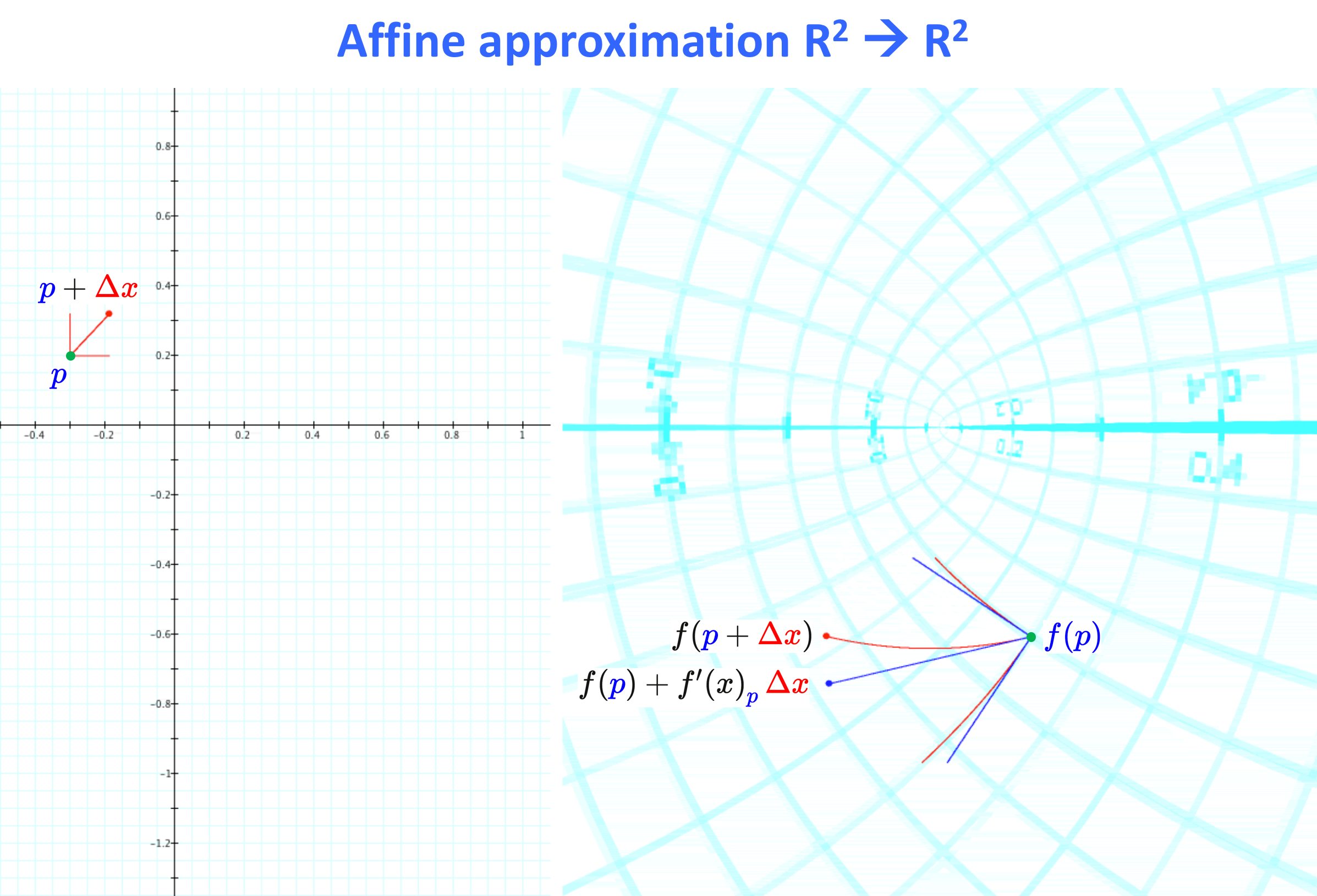
Affine approximation from 2D to 2D
The affine approximation of a differentiable function \, f : {\mathbb{R}}^2 \rightarrow {\mathbb{R}}^2
A function from (part of) \, {\mathbb{R}}^2 \rightarrow {\mathbb{R}}^2 :
\, f(x) = f(x_1, x_2) = (f_1(x_1, x_2), f_2(x_1, x_2)) \, .
The affine approximation of a differentiable function \, f : \mathbb{R}^2 \rightarrow \mathbb{R}^2 \,
in the neighborhood of a point \, \textcolor{blue}{p} = (\textcolor{blue}{p_1}, \textcolor{blue}{p_2}) \, \in {\mathbb{R}}^2 \, is defined by
\, f_{\textcolor{blue}{p}}(x) \stackrel{\text{def}}{=} f(\textcolor{blue}{p}) + {f'(x)}_{\textcolor{blue}{p}} \, (x - \textcolor{blue}{p}) \, \equiv \, f(\textcolor{blue}{p}) + {f'(x)}_{\textcolor{blue}{p}} \, \textcolor{red} {\Delta x} .
The characteristic property of the affine approximation \, f_{\textcolor{blue}{p}} \, can be expressed as:
\, f(x) = f_{\textcolor{blue}{p}}(x) + o(|x - \textcolor{blue}{p}|) \, when \, x \, is close enough to \, \textcolor{blue}{p} .
In matrix algebra this can be expressed as:
\, \begin{pmatrix} f_1(\textcolor{blue}{p} + \textcolor{red}{\Delta x}) \\ f_2(\textcolor{blue}{p} + \textcolor{red}{\Delta x}) \end{pmatrix} = \begin{pmatrix} f_1(\textcolor{blue}{p}) \\ f_2(\textcolor{blue}{p}) \end{pmatrix} + {\begin{pmatrix} \frac{\partial f_1}{\partial x_1} & \frac{\partial f_1}{\partial x_2} \\ \frac{\partial f_2}{\partial x_1} & \frac{\partial f_2}{\partial x_2} \end{pmatrix}}_{\textcolor{blue}{p}} \, \begin{pmatrix} \textcolor{red}{\Delta x_1} \\ \textcolor{red}{\Delta x_2} \end{pmatrix} + \begin{pmatrix} o( | \textcolor{red}{\Delta x} | ) \\ o( | \textcolor{red}{\Delta x} | ) \end{pmatrix} \, = \, = \, \begin{pmatrix} f_1(\textcolor{blue}{p}) \\ f_2(\textcolor{blue}{p}) \end{pmatrix} + \begin{pmatrix} {\frac{\partial f_1}{\partial x_1}}_{\textcolor{blue}{p}} \, \textcolor{red}{\Delta x_1} + {\frac{\partial f_1}{\partial x_2}}_{\textcolor{blue}{p}} \, \textcolor{red}{\Delta x_2} + o( | \textcolor{red}{\Delta x} | ) \\ {\frac{\partial f_2}{\partial x_1}}_{\textcolor{blue}{p}} \, \textcolor{red}{\Delta x_1} + {\frac{\partial f_2}{\partial x_2}}_{\textcolor{blue}{p}} \, \textcolor{red}{\Delta x_2} + o( | \textcolor{red}{\Delta x} | ) \end{pmatrix}///////
A devil transformed by \, e^{z + \textcolor{red}{p}} \, :
///////
Affine approximation of \, f(F(x,y), G(x,y)) \,
where \, F(x, y) = x^2 - y^2 \, , \, G(x, y) = 2 x y \,
///////
Conformal mapping :: z^2 – square grid.
Drag the purple point to move the grid.
(Ron Avitzur on the Graphing Calculator)
///////
/// Connect with Optical Properties of Conics.
Complex squaring takes a rectangular grid to confocal parabolas:

The interactive simulation that created this movie
///////
Affine approximation from 3D to 3D
The affine approximation of a differentiable function \, f : {\mathbb{R}}^3 \rightarrow {\mathbb{R}}^3
\, f(x) = f(x_1, x_2, x_3) = (f_1(x_1, x_2, x_3), f_2(x_1, x_2, x_3), f_3(x_1, x_2, x_3)) \, .
The affine approximation of a differentiable function \, f : \mathbb{R}^3 \rightarrow \mathbb{R}^3 \,
in the neighborhood of a point \, \textcolor{blue}{p} = (\textcolor{blue}{p_1}, \textcolor{blue}{p_2}, \textcolor{blue}{p_3}) \, \in {\mathbb{R}}^3 \, is defined by
\, f_{\textcolor{blue}{p}}(x) \stackrel{\text{def}}{=} f(\textcolor{blue}{p}) + {f'(x)}_{\textcolor{blue}{p}} \, (x - \textcolor{blue}{p}) \, \equiv \, f(\textcolor{blue}{p}) + {f'(x)}_{\textcolor{blue}{p}} \, \textcolor{red} {\Delta x} .
The characteristic property of the affine approximation \, f_{\textcolor{blue}{p}} \, can be expressed as:
\, f(x) = f_{\textcolor{blue}{p}}(x) + o(|x - \textcolor{blue}{p}|) \, when \, x \, is close enough to \, \textcolor{blue}{p} .
In matrix algebra this can be expressed as:
\, \begin{pmatrix} f_1(\textcolor{blue}{p} + \textcolor{red}{\Delta x}) \\ f_2(\textcolor{blue}{p} + \textcolor{red}{\Delta x}) \\ f_3(\textcolor{blue}{p} + \textcolor{red}{\Delta x}) \end{pmatrix} = \begin{pmatrix} f_1(\textcolor{blue}{p}) \\ f_2(\textcolor{blue}{p}) \\ f_3(\textcolor{blue}{p}) \end{pmatrix} + {\begin{pmatrix} \frac{\partial f_1}{\partial x_1} & \frac{\partial f_1}{\partial x_2} & \frac{\partial f_1}{\partial x_3} \\ \frac{\partial f_2}{\partial x_1} & \frac{\partial f_2}{\partial x_2} & \frac{\partial f_2}{\partial x_3} \\ \frac{\partial f_3}{\partial x_1} & \frac{\partial f_3}{\partial x_2} & \frac{\partial f_3}{\partial x_3} \end{pmatrix}}_{\textcolor{blue}{p}} \, \begin{pmatrix} \textcolor{red}{\Delta x_1} \\ \textcolor{red}{\Delta x_2} \\ \textcolor{red}{\Delta x_3} \end{pmatrix} + \begin{pmatrix} o(| \textcolor{red}{\Delta x} | \\ o( | \textcolor{red}{\Delta x} | \\ o( |\textcolor{red}{\Delta x} | \end{pmatrix}///////
Affine Approximation in 3D:
The interactive simulation that created this movie
///////