This page is a sub-page of our page on Non-Euclidean Geometry.
///////
The sub-pages of this page are:
• The Beltrami-Klein model of Hyperbolic Geometry
• The Riemann-Poincaré model of Hyperbolic Geometry
///////
Related KMR pages:
• Elliptic geometry
• Euclidean geometry
• Projective geometry
• Projective metrics
• The Euclidean degeneration
///////
Books:
• Felix Klein (1926), Vorlesungen über Nichteuklidische Geometrie,
Verlag von Julius Springer in Berlin, (1928).
• Jürgen Richter-Gebert (2011), Perspectives on Projective Geometry – A Guided Tour Through Real and Complex Geometry, Springer, ISBN 978-3-642-17285-4.
• D.M.Y. Sommerville (1914), The Elements of Non-Euclidean Geometry, Dover (1958, 2005).
• Henry Parker Manning (1901), Introductory Non-Euclidean Geometry, Dover (1963, 2005).
• H.S.M. Coxeter (1947 (1942)), Non-Euclidean Geometry.
• W. T. Fishback (1969), Projective and Euclidean Geometry, John Wiley & Sons, Inc.,
ISBN 13: 978-047126-053-0.
• John Stillwell (2016), Elements of Mathematics – From Euclid to Gödel,
Princeton University Press, ISBN 978-0-691-17854-7.
• John Stillwell (1999, (1989)), Mathematics and Its History, Springer, ISBN 0-387-96981-0.
• Jeremy Gray (2007), Worlds Out of Nothing – A Course in the History of Geometry in the 19th Century, Springer, ISBN 1-84628-632-8.
///////
Other relevant sources of information:
• Hyperbolic geometry
• Hyperbolic triangle
• Hyperbolic circles and discs
• Hyperbolic functions
• Getting Into Shapes: From Hyperbolic Geometry to Cube Complexes and Back,
by Erika Klarreich in Quanta Magazine.
• Non-Euclidean Geometry
• Illuminating hyperbolic geometry
• Hypercycle Geometry
• Riemann-Poincaré Hyperbolic Disc
• Horocycle
• Apeirogon
• Konrad Polthier hyperboloid model
• Google images for Konrad Polthier hyperboloid model
• Piece for triple piano in hyperbolic space (by Vi Hart and Henry Segerman)
• Coordinate systems for the hyperbolic plane
• Area of an hyperbolic triangle made by two geodesic and a horocycle
• Hyperbolic angle
• Tractrix
• Catenary
• Comparison between circular and hyperbolic angles
• Hyperbolic and circular angles
///////
The interactive simulations on this page can be navigated with the Free Viewer
of the Graphing Calculator.
///////
A hyperbolic yardstick:
The interactive simulation that created this movie.
///////
On the hyperbolic line (shown in the simulation), the distance between any two neighboring points is the same. In German this type of arrangement is called a “Schrittmass” (= a “step-measure”). The length of each step is determined by a suitable choice of a multiplicative constant. In general, “hyperbolic infinity” can be represented by any real conic.
In the hyperbolic plane shown in the simulation above,
infinity is represented by both branches of the (blue) hyperbola
and, on the (blue) hyperbolic line, infinity is represented by the two red points.
These two infinite points on the hyperbolic line are identical to
the points of intersection of this line with the asymptotes of the infinite hyperbola.
It follows that the distance from any one of the black points on the line to any one of the two red points is infinite. These (red) infinite points cannot be reached, no matter how far you extend the yardstick.
APPLICATION :
The Minkowski SpaceTime geometry is a geometry that is well suited to represent the measurements of different inertial observers (= observers moving with constant velocity relative to each other) according to Einstein’s special theory of relativity.
In Minkowski geometry, the asymptotes of the hyperbola seen above correspond to a plane of intersection through the light-cone. This plane passes through “the origin”, and the origin itself corresponds to the “standard event”, an event that is used to calibrate two inertial observers in a so-called “standard configuration”.
In 1-dimentional relativity theory, the asymptotes themselves correspond to the light-cone and the branch of the hyperbola shown above corresponds to the future, while the other branch corresponds to the past.
If one of the inertial observers will find her measurements to fit a certain branch of the hyperbola, so will the other observer.
Hence this branch of the hyperbola represents the “curve of agreements” between two inertial observers.
It also represents the “curve of possible agreements” between these observers and ALL OTHER inertial observers (that are calibrated in the standard configuration with respect to the first two inertial observers).
The only thing they can all agree on is whether the observed event occurred in the future (= on the future branch of the hyperbola) or in the past (= on the past branch of the hyperbola).
If, on the other hand, the hyperbola lies outside the light-cone, then the observers will not (in general) be able to agree whether the corresponding event occurred in the future or in the past.
Hence, in special relativity theory, such an hyperbola is referred to as a “curve of elsewhere”.
(See “Einstein for Linelanders” at https://kmr.dialectica.se/wp/research/math-rehab/first-class-mathematics/short-circuiting-learning-objects/stories/einstein-for-linelanders/ ).
In 2-dimensional relativity theory, the 2-d representation can be created by rotating the 1-d representation around its line of symmetry. Then the two asymptotes generate a circular cone (= the light-cone) and the hyperbola generates a hyperboloid of revolution.
If this hyperboloid has two sheets (= different parts), one of these sheets corresponds to the future (in relation to the standard event), while the other sheet corresponds to the past.
If one of the inertial observers will find her measurements to fit a certain one of the two sheets of this hyperboloid, so will the other observer.
Hence each sheet of a two-sheeted hyperboloid represents the “surface of agreement” between the measurements of two different inertial observers.
It also represents the “surface of possible agreements” between them and ALL OTHER inertial observers (that are calibrated in the standard configuration with respect to the first two inertial observers).
The only thing they can all agree on is whether the observed event occurred in the future (= on the future sheet of the hyperboloid) or in the past (= on the past sheet of the hyperboloid).
If, on the other hand, the hyperboloid has only one sheet, then the hyperboloid is connected (= has no separate sheets) and lies outside the light-cone. In this case, the observers will not (in general) be able to agree whether the corresponding event occurred in the future or in the past.
Hence, in special relativity theory, a one-sheeted hyperboloid is referred to as a “surface of elsewhere”.
(See Einstein for Flatlanders at https://kmr.dialectica.se/wp/research/math-rehab/first-class-mathematics/short-circuiting-learning-objects/stories/einstein-for-flatlanders/ )
///////
The circular sector \, ( \cos \theta \, , \sin \theta ) \, and the hyperbolic sector \, ( \cosh \theta \, , \sinh \theta ) \,
have equal areas since each of them has the (euclidean) area \, \theta/2 \, :
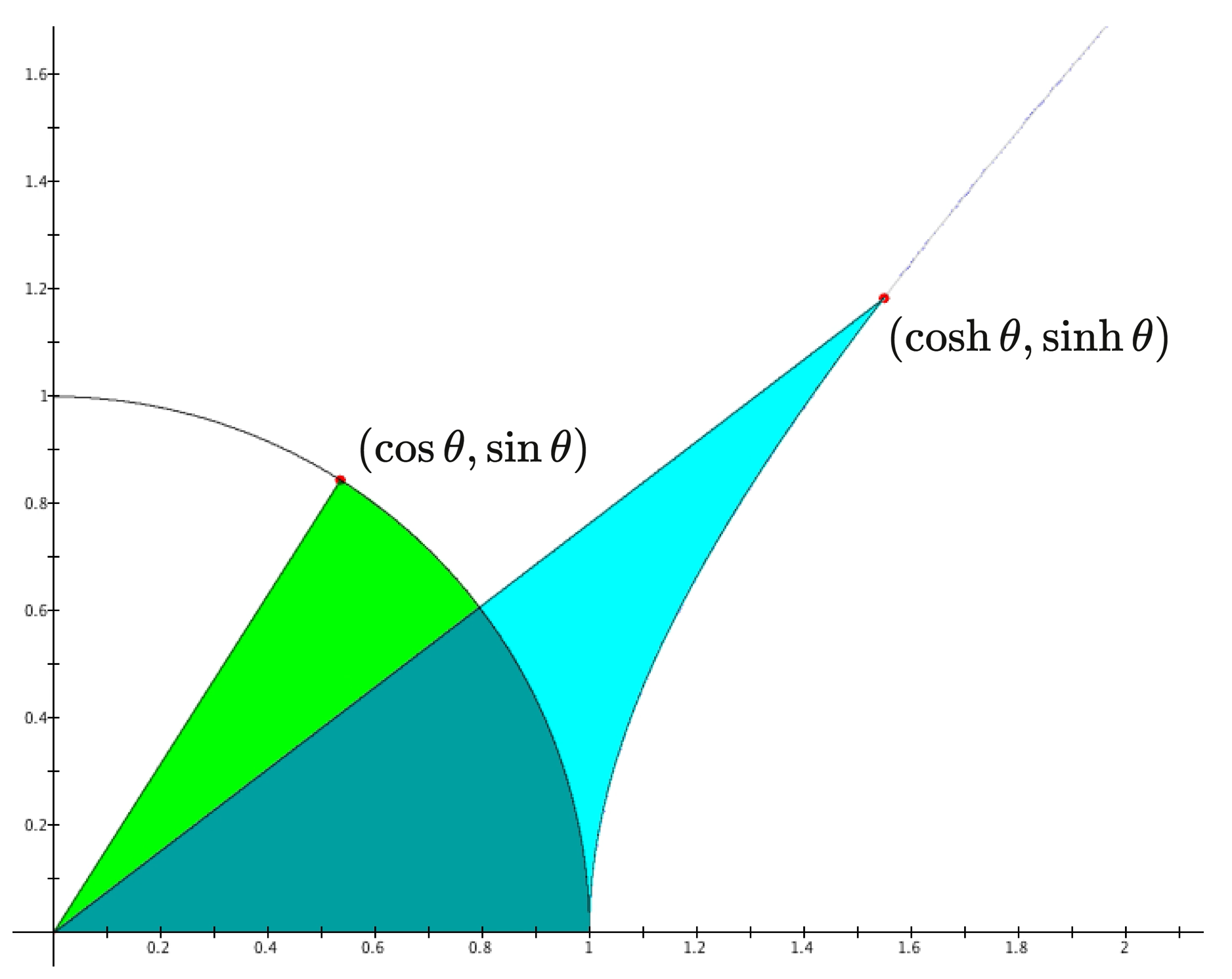
The red point on the unit circe is given by \, (\cos \theta, \sin \theta) \, , and
the red point on the unit hyperbola is given by \, (\cosh \theta, \sinh \theta) \, .
The circular sector area (green + bluegreen) is equal to the hyperbolic sector area
(blue + bluegreen), since both areas are equal to \, \theta/2 \, .
Hyperbolic and circular angles at Wikimedia.
///////
Comparison between a euclidean and a hyperbolic angular yardstick:
(An angular yardstick is better known as a protractor)
The correspondence between the same-coloured points depicted above connects the point \, ( \cos (n * \Delta \theta) , \sin (n * \Delta \theta) ) \, and the point \, ( \cosh (n * \Delta \theta), \sinh (n * \Delta \theta) ) .
Hence, as \, n \, increases, all the six points are ‘jumping’ with the same angular shift \, \Delta \theta \, .
FACT: Each of the four sector areas formed by the neighboring points shown in the film
is equal to \, \Delta \theta / 2 \, , independently of the value of \, n \, .
This fact forms the basis for comparisons between the euclidean and the hyperbolic concept of “equality-of-angle.”
Euclidean protractor:
\, \cos(\theta) \, \equiv \, \frac{1}{2} (e^{i \, \theta} + e^{-i \, \theta} ) \, ,
\, \sin(\theta) \, \equiv \, \frac{1}{2i} (e^{i \, \theta} - e^{-i \, \theta} ) \,
Hyperbolic protractor:
\, \cosh(\theta) \, \equiv \, \cos(i \, \theta) \, \equiv \, \frac{1}{2} (e^{i^2 \, \theta} + e^{- i^2 \, \theta} ) \, \equiv \, \frac{1}{2} (e^{\theta} + e^{-\theta} ) \, ,
\, \sinh(\theta) \, \equiv \, - i \, \sin(i \, \theta) \, \equiv \, -i \, \frac{1}{2i} (e^{i^2 \, \theta} - e^{-i^2 \, \theta} ) \, \equiv \, \frac{1}{2} (e^{ \theta} - e^{- \theta} ) \,
///////
\, \cosh(i \, \theta) \, \equiv \, \frac{1}{2} (e^{i \, \theta} + e^{- i \, \theta} ) \, \equiv \, \cos(\theta) \, ,
\, \sinh(i \, \theta) \, \equiv \, \frac{1}{2} (e^{ i \, \theta} - e^{- i \, \theta} ) \, \equiv \, i \, \sin(\theta) \,
///////
Hyperbolic circles and cycles:
///////
Concentric circles with fixed center (inside the hyperbolic space)
and varying radius (in the Beltrami-Klein model):
///////
Concentric horocycles with fixed center (at infinity)
and varying radius (in the Beltrami-Klein model):
///////
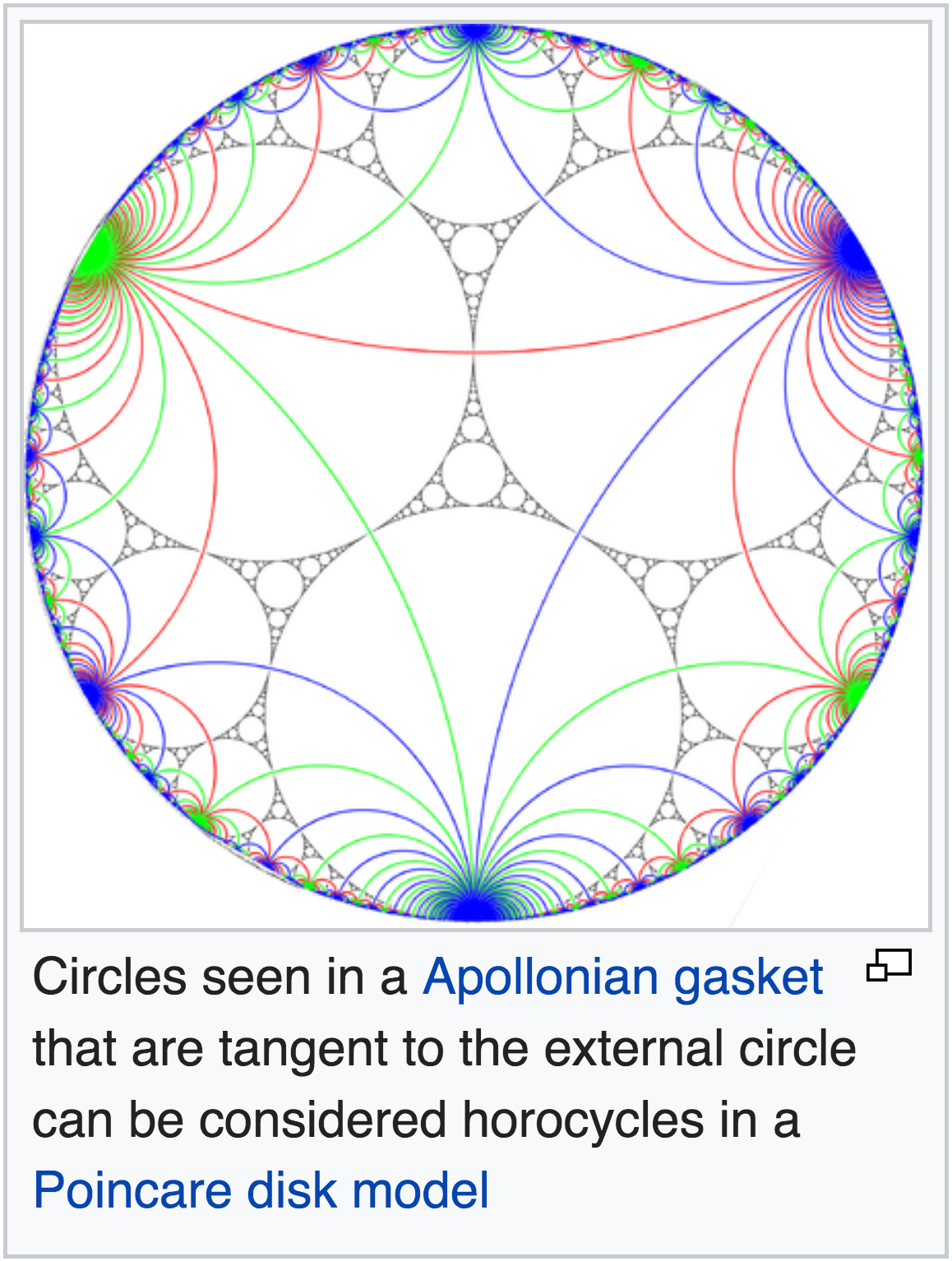
Horocycle in the Riemann-Poincaré model:

Horocycles in an Appolonian gasket:
///////
Concentric hypercycles with fixed center (outside the hyperbolic space)
and varying radius (in the Beltrami-Klein model):
///////
Here is a link to the interactive simulation that created the three videos on concentric circles and cycles appearing above.
///////
Hyperbolic circle/cycle with varying center and radius
(in the Beltrami-Klein model):
///////
Pappus-Pascal’s theorem:
///////
Isometry of a non-degenerated geometry:
///////
Escher’s Angels and Devils moving in the Riemann-Poincaré disk
(MathRehab on YouTube):
///////
M.C. Escher’s use of Hyperbolic Space
///////
“Heaven and Hell” in hyperbolic space
(Vladimir Bulatov on YouTube):
///////
Visualizing the sphere and the hyperbolic plane
(five projections of each):
Hyperbolic Geometry is Projective Relativistic Geometry
(full lecture by N.J. Wildberger):
///////
Wild Linear Algebra 34: Oriented circles and 3D relativistic geometry I:
Universal Hyperbolic Geometry 1: Apollonius and polarity
(by N.J. Wildberger):
///////
Illuminating Hyperbolic Geometry:
///////
Amber Case – An Introduction to Hyperbolic Geometry:
hyperbolical:
Hyperbolic Geometry in Art:
Triangular tilings in hyperbolic, euclidean, and elliptic geometry:
Triangular tilings in hyperbolic, euclidean, and elliptic geometry
///////
Bill Thurston and the Geometry Center on YouTube:
Not Knot (Part 1/2):
Not Knot (Part 2/2):
///////
/////////////////////////////////
/////////////////////////////////
Mathematical context
In Transcendental Curves in the Leibnizian Calculus, 2017
4.4.7 Conclusion
Considering Johann Bernoulli’s lectures as a whole, we may observe an overarching conflict between general, abstract methods and concrete, specific geometry. Bernoulli shows a clear preference for obtaining solutions with a direct geometrical meaning as opposed to mere abstract formulas. This is perfectly understandable since, to Bernoulli and his contemporaries, the calculus is a method for advancing geometry rather than a self-contained analytical game. It is not enough that the calculus can incorporate geometrical and physical problems and generate answers in a language internal to itself, such as differential equations and complicated integrals. It is judged rather by the geometrical end product it can generate from these expressions. And the conditions under which the desired end product is produced are quite unmistakable: abstract method, abstract answer; geometry in, geometry out.
Thus, for instance, general analytic methods are often vastly inferior in specific cases to ad hoc methods respecting the intrinsic geometry of the curve. Examples include the general formulas for arc length, involute rectification, and caustics, as well as brute-force integration generally, all of which are abandoned more often than not by Bernoulli in specific cases. Indeed, curves characterised in geometrical terms (cycloids, spirals, involutes, envelopes, etc.) tend to be eminently treatable by more tailored methods and yield simple, geometrically interpretable answers, whereas when curves are treated analytically the calculations often become unfeasible (as often happens with arc length integrals, for example) or lead to unilluminating results (such as in the case of the tangent of the cissoid).
Further strengthening this dichotomy is the tendency for the set of geometrically elegant curves (such as cycloids, spirals, etc.) to be closed under geometrically elegant operations (such as evolutes, involutes, caustics, etc.). Jacob Bernoulli (1692) observed much the same thing and was so impressed with it that he later had the logarithmic spiral—the “spira mirabilis,” as he called it—engraved on his tombstone with the inscription “eadem mutata resurgo” (“[although] changed, I appear again the same”), referring to this curve’s property of being its own caustic, its own evolute, etc. (cf. Section 4.4.4.4).
Even more remarkably, simple and elegant geometry tends to be admirably applicable; one might call it an “unreasonable effectiveness,” to borrow the famous phrase of Wigner (1960). For instance, the simple geometrical idea of the involute is remarkably powerful for rectifying curves (again, often superior to the brute-force analytical method). And curves with simple geometrical definitions again and again turn out to have physical applications, such as the cycloid as the isochrone, or the epicycloid as the caustic.
Altogether, these kinds of examples suggest that geometry possesses a sort of self-sufficiency. They provide ample reason for one to dream of a utopia in which geometrically elegant problems have geometrically elegant solutions. Indeed, the most undisputed geometrical masters, such as Archimedes and Huygens, always seemed to pluck their finest fruits from this utopia. It is understandable, then, for this to be considered the mark of a truly great geometer. And consequently it is understandable also that abstract and general analytical methods and results will have a hard time finding justification in such a setting.