This page is a sub-page of our page on New Foundations for Classical Mechanics.
///////
Related KMR-pages:
• Chapter 1: Origins of Geometric Algebra
• Chapter 2: Developments in Geometric Algebra
• Chapter 4: Central Forces and Two-Particle Systems
///////
Books:
• René Descartes (1637), La Géometrie
• Hermann Günther Graßmann (1844), Die Lineale Ausdehnungslehre, ein neuer Zweig der Mathematik
• A New Branch Of Mathematics – The Ausdehnungslehre of 1844 and Other Works, translated by Lloyd C. Kannenberg (1995)
• William Kingdon Clifford (1878), Applications of Grassmann’s Extensive Algebra, American Journal of Mathematics Vol. 1, No. 4 (1878), pp. 350-358 (9 pages), Published by: The Johns Hopkins University Press
• David Hestenes (1993, (1986)), New Foundations for Classical Mechanics
///////
Other relevant sources of information:
///////
/////// Quoting Hestenes (1986): New Foundations for Classical Mechanics (Chapter 3):
Chapter 3: Mechanics of a Single Particle
Table Of Content
///////
3-1. Newton’s Program
3-2. Constant Force
3-3. Constant Force With Linear Drag
///////
In this chapter we learn how to use geometric algebra to describe and analyze the motion of a single particle. From a physical point of view, we will be concerned with constructing the simplest models for a physical system and discussing their applications and limitations. From a mathematical point of view we will be concerned with solving the simplest second order vector differential equations and analyzing the the geometrical properties of solutions.
Most of the results of Chapter 2 will be used in this chapter in one way or another. Of course, the main mathematical tool will be the geometric algebra of physical space. Since the reader is presumed to have some familiarity with mechanics already, a number of basic terms and concepts will be used with no more than the briefest introduction. A critical and systematic analysis of the foundations of mechanics will be undertaken in Chapter 9. General methods for solving differential equations will be developed as they are needed.
Although only the simplest models and differential equations are considered in this chapter, the results should not be regarded as trivial, for the simple models provide the starting point for the analyzing and solving of complex problems. Consequently, the time for developing an elegant formulation and thorough analysis of simple models is time well spent.
3-1. Newton’s Program
Isaac Newton (1642 – 1727) is rightly regarded as the founder of the science called mechanics. Of course, he was neither the first nor the last to make important contributions to the subject. He deserves the title of “founder”, because he integrated the insights of his predecessors into a comprehensive theory. Furthermore, he inaugurated a program to refine and extend that theory by systematically investigating and classifying the properties of all physical objects. Newtonian mechanics is, therefore, more than a particular scientific theory; it is a well-defined program of research into the structure of the physical world.
This section reviews the major features of Newtonian mechanics as it stands today. Naturally, a modern formulation of mechanics differs somewhat from Newton’s but this is not the place to trace the intricacies of its evolution. Also, for the time being we take the fundamental concepts of space and time for granted, just as Newton did in his Principia. It will not be profitable to wrestle with subtleties in the foundation of mechanics until some proficiency with the mathematical formalism has been developed, so we delay the attempt until Chapter 9.
The grand goal of Newton’s program is to describe and explain all properties of all physical objects. The approach of the program is determined by two general assumptions: first, that every physical object can be represented as a composite of particles; second, that the behavior of a particle is governed by interactions with other particles. The properties of a physical object, then, are determined by the properties of its parts. For example, structural properties of an object, such as rigidity or plasticity, are determined by the interactions among its parts. The program of mechanics is to explain the diverse properties of objects in our experience in terms of a few kinds of interactions among a few kinds of particles.
The great power of Newtonian mechanics is achieved by formulating the generalities of the last paragraph in specific mathematical terms. It depends on a clear formulation of the key concepts: particle and interaction. A particle is understood to be an object with a definite orbit in space and time. The orbit is represented by a function \, \bold x = \bold x (t) \, which specifies the particle’s position \, \bold x \, at each time \, t . To express the continuous existence of the particle in some interval of time, the function \, \bold x = \bold x (t) \, must be a continuous function of the variable \, t \, in that interval. When specified for all times in an interval, the function \, \bold x = \bold x (t) \, describes a motion of the particle.
The central hypothesis of Newtonian mechanics is that variations in the motion of a particle are completely determines by its interactions with other particles. More specifically, the motion is determined by an equation of the general form
\, \bold f = m \, \ddot{\bold x} \;\;\;\;\;\;\;\;\;\;\;\;\;\;\;\;\;\;\;\;\;\;\;\;\;\;\;\;\;\;\;\;\;\;\;\;\;\;\;\;\;\;\;\;\;\;\;\;\;\;\;\;\;\;\;\;\;\;\;\;\;\;\;\;\;\;\;\;\;\;\;\;\;\;\;\;\;\;\;\;\;\;\;\;\;\;\; (1.1)
where \, \ddot{\bold x} \, is the acceleration of the particle, the scalar \, m \, is a constant called the mass of the particle, and the force \, \bold f \, expresses the influence of other particles. This hypothesis is commonly referred to as “Newton’s second law of motion”, though it was Euler who finally cast it in the form we use today.
Newton’s Law (1.1) becomes a definite differential equation determining the motion of a particle only when the force \, \bold f \, is expressed as a specific function of \, \bold x (t) \, and its derivatives. With this much understood, the thrust of Newton’s program can be summarized by the dictum: focus on the forces. This should be interpreted as an admonition to study the motions of physical objects and find forces of interaction sufficient to determine those motions. The aim is to classify the kinds of forces and so develop a classification of particles according to the kinds of interactions in which they participate. The classification is not complete today, but it has been carried a long way.
Newton’s program has been so successful largely because it has proved possible to account for the motions of physical objects with forces of simple mathematical form. The “forces of nature” appear to have two properties of such universality that they should be regarded as laws, though they were not identified as such by Newton. We shall refer to them as the principles of additivity and analyticity.
According to the principle of additivity (or superposition) of forces, the force \, \bold f \, on a given particle can be expressed as the vector sum of forces \, {\bold f}_k \, independently exerted by each particle with which it interacts, that is
\, \bold f = {\bold f}_1 + {\bold f}_2 + \cdots = \sum\limits_{k} {\bold f}_k \, . \;\;\;\;\;\;\;\;\;\;\;\;\;\;\;\;\;\;\;\;\;\;\;\;\;\;\;\;\;\;\;\;\;\;\;\;\;\;\;\;\;\;\;\;\;\;\;\;\;\;\;\;\;\;\;\;\;\; (1.2)
This principle enables us to isolate and study different kinds of forces independently as well as to reduce complex forces to a superposition of simple forces. Newton’s program could hardly have progressed without it.
According to the principle of analyticity (or continuity), the force of one particle on another is an exclusive, analytic function of the positions and velocities of both particles. The adjective “exclusive” means that no other variables are involved. The adjective “analytic” means that the function is smoothly varying in the sense that derivatives (with respect to time) of all orders have finite values. The principle of analyticity implies that the force \, \bold f \, on a particle with position \, \bold x = \bold x (t) \, and velocity \, \dot {\bold x} = \dot {\bold x} (t) \, is always an analytic function
\, \bold f = \bold f ( \bold x, \dot{\bold x}, t ), \;\;\;\;\;\;\;\;\;\;\;\;\;\;\;\;\;\;\;\;\;\;\;\;\;\;\;\;\;\;\;\;\;\;\;\;\;\;\;\;\;\;\;\;\;\;\;\;\;\;\;\;\;\;\;\;\;\;\;\;\;\;\;\;\;\;\;\;\;\;\;\;\;\;\;\;\; (1.3)
where the explicit time dependence arises from motions of the particles determining the force. Notice that the force is not a function of \, \ddot{\bold x} \, and higher order derivatives. An exception to this rule is the so-called “radiative reaction force” which requires special treatment that we cannot go into here. Mathematical idealizations or approximations that violate the analyticity principle are often useful, as long as their ranges of validity are understood.
//// FORTSÄTT HÄR
3-2. Constant Force
In this section we study the motion of a particle subject to a constant gravitational force \, \bold f = m \, \ddot{\bold g} . Of course, our results describe the motion of a particle with charge \, q \, in a constant electric field \, \bold E \, just as well; it is only necessary to write \, \bold g = \frac{q}{m} \bold E \, for the electrical force per unit mass.
According to the fundamental law of mechanics, a particle subject to a constant force undergoes a constant acceleration. For a force per unit mass \, \bold g , the particle trajectory \, \bold x = \bold x (t) \, is determined by the differential equation
\, \ddot{\bold x} = \dot{\bold v} = \bold g \;\;\;\;\;\;\;\;\;\;\;\;\;\;\;\;\;\;\;\;\;\;\;\;\;\;\;\;\;\;\;\;\;\;\;\;\;\;\;\;\;\;\;\;\;\;\;\;\;\;\;\;\;\;\;\;\;\;\;\;\;\;\;\;\;\;\;\;\;\;\;\;\;\;\;\;\;\;\;\;\;\;\; (2.1)
subject to the initial conditions
\, \dot{\bold x}(0) = {\bold v}(0) = {\bold v}_0, \;\;\;\;\;\;\;\;\;\;\;\;\;\;\;\;\;\;\;\;\;\;\;\;\;\;\;\;\;\;\;\;\;\;\;\;\;\;\;\;\;\;\;\;\;\;\;\;\;\;\;\;\;\;\;\;\;\;\;\;\;\;\;\;\;\;\;\;\;\, (2.2a)
\, {\bold x}(0) = {\bold x}_0. \;\;\;\;\;\;\;\;\;\;\;\;\;\;\;\;\;\;\;\;\;\;\;\;\;\;\;\;\;\;\;\;\;\;\;\;\;\;\;\;\;\;\;\;\;\;\;\;\;\;\;\;\;\;\;\;\;\;\;\;\;\;\;\;\;\;\;\;\;\;\;\;\;\;\;\;\;\;\;\;\; (2.2b)
Using (2-7.19) and (2-7.17), Equation (2.1) can be integrated directly to get the velocity \, \bold v = \bold v (t) \, at any time \, t ; thus
\, \dot{\bold x} = \bold v = \bold g \, t + {\bold v}_0. \;\;\;\;\;\;\;\;\;\;\;\;\;\;\;\;\;\;\;\;\;\;\;\;\;\;\;\;\;\;\;\;\;\;\;\;\;\;\;\;\;\;\;\;\;\;\;\;\;\;\;\;\;\;\;\;\;\;\;\;\;\;\;\;\;\;\;\;\;\;\; (2.3)
A second integration gives
\, \bold r = \bold x - {\bold x}_0 = \frac {1}{2} \bold g \, t^2 + {\bold v}_0 \, t. \;\;\;\;\;\;\;\;\;\;\;\;\;\;\;\;\;\;\;\;\;\;\;\;\;\;\;\;\;\;\;\;\;\;\;\;\;\;\;\;\;\;\;\;\;\;\;\;\;\;\;\;\;\;\;\;\;\; (2.4)
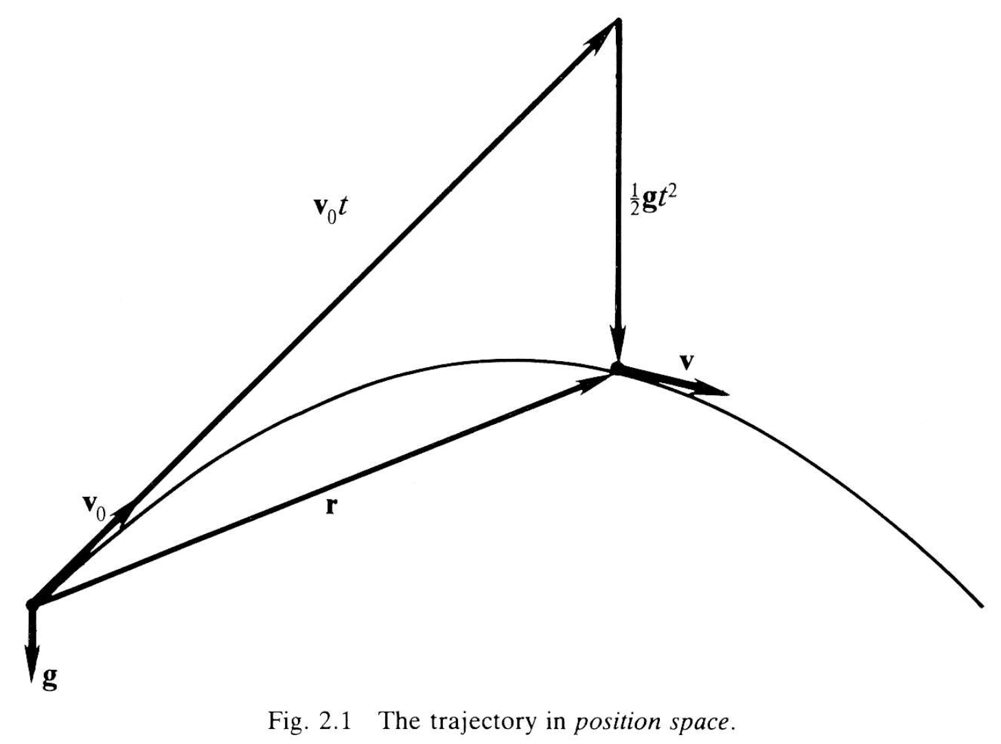
Fig. 2.1.
This is a parametric equation for the displacement of the particle as a function of time. The trajectory is a segment of a parabola, as shown in Figure 2.1. The solution (2.4) presents the parabolic motion of the particle as the superposition of two linear motions. The term \, {\bold v}_0 \, t \, can be interpreted as the displacement of a point at rest in a reference system moving with velocity \, {\bold v}_0 , while the term \, \frac {1}{2} \bold g \, t^2 \, is interpreted as the displacement of the particle initially at rest in the moving system.
Accordingly, the constants in (2.4) determine a “natural” coordinate system for locating the particle at any time; the origin is determined by \, {\bold x}_0 , while coordinate directions and scales are given by the vectors \,{\bold v}_0 \, and \bold g . This is a skew coordinate system, but the particle’s natural position coordinates \, t \, and \, \frac {1}{2} \bold g \, t^2 \, are obviously quadratically related, just as they are in the familiar representation by rectangular coordinates.
Mathematically speaking the quantity \, \frac {1}{2} \bold g \, t^2 \, is a particular solution of the equation of motion (2.1), while \, {\bold v}_0 \, t + {\bold x}_0 \, is the general solution of the homogeneous differential equation \, \ddot{\bold x} = 0 .
The description of motion can be simplified by representing it in velocity space instead of position space. A curve traced by the velocity \, \bold v = \bold v (t) \, is called a hodograph. According to (2.3), the hodograph of a particle subject to a constant force is a straight line. In velocity space the location of the particle can be represented by the average velocity \, \overline{\bold v} = \overline{\bold v} (t) . The parametric equation for \, \overline{\bold v} \, is obtained by writing (2.4) in the form
\, \overline{\bold v} = \dfrac{\bold r}{t} = \frac{1}{2} {\bold g} \, t + {\bold v}_0. \;\;\;\;\;\;\;\;\;\;\;\;\;\;\;\;\;\;\;\;\;\;\;\;\;\;\;\;\;\;\;\;\;\;\;\;\;\;\;\;\;\;\;\;\;\;\;\;\;\;\;\;\;\;\;\;\;\;\;\;\;\;\;\;\;\;\;\; (2.5)
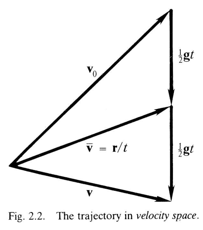
Fig. 2.2.
As illustrated in Figure 2.2, the trajectory \, \overline{\bold v} (t) \, is simply a vertical straight line beginning at {\bold v}_0 . Figure 2.2 also shows the simple relation of the average velocity (2.5) to the actual velocity (2.3), a relation which is disguised if the equation for displacement (2.4) is used directly. Figure 2.2 contains all the information about the projectile motion, so all questions about the motion can be answered by solving the triangles in the figure, graphically or algebraically, for the relevant variables. Let us see how to do this efficiently.
Projectile Range
Although the displacement \, r = | \, \bold r \, | \, is represented only indirectly in velocity space, it is nonetheless easy to compute. Consider, for example, the problem of determining the range \, r \, of a target sighted in a direction \, \hat{\bold r} , which has been hit by a projectile launched with velocity \, {\bold v}_0 . This problem can easily be solved by the graphical method illustrated in Figure 2.2, assuming, of course, that the flight of the projectile is adequately represented as that of a particle with constant acceleration \, \bold g . The method simply exploits properties of Figure 2.2.
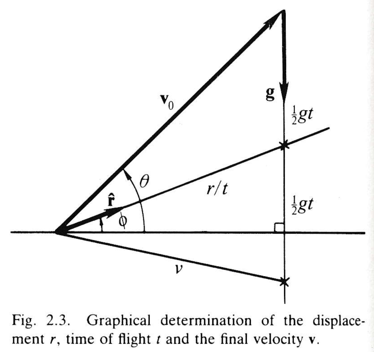
Fig. 2.3.
Having “laid out” \, {\bold v}_0 \, on graph paper, as indicated in Figure 2.3, one extends a line from the base of \, {\bold v}_0 \, in the direction \, \hat{\bold r} \, to its intersection with a vertical line extending from the tip of \, {\bold v}_0 . The lengths of the two sides of the triangle thus constructed are then measured to get the values of \, \frac{1}{2} g \, t \, and \, \dfrac{r}{t} , from which one can compute \, r \, and \, t \, as well, if desired. Figure 2.2 also shows how the construction can be extended to determine the final velocity \, \bold v \, of the projectile. Angles with the horizontal are indicated in Figure 2.2, since they are commonly used to specify relative direction in practical problems.
The same problem can be solved by algebraic means. Outer multiplication of (2.5) by \, \bold r \, produces \frac{1}{2} t \, \bold g \wedge \bold r = \bold r \wedge {\bold v}_0 .
Hence
\, t = \dfrac{ 2 \hat{\bold r} \wedge {\bold v}_0 }{ \bold g \wedge \hat{\bold r} } = \dfrac{ 2 v_0 }{ g } \dfrac{ | \, \hat{\bold r} \wedge \hat{\bold v}_0 \, | }{ | \, \hat{\bold g} \wedge \hat{\bold r} \, | } . \, \;\;\;\;\;\;\;\;\;\;\;\;\;\;\;\;\;\;\;\;\;\;\;\;\;\;\;\;\;\;\;\;\;\;\;\;\;\;\;\;\;\;\;\;\;\;\;\;\;\;\;\;\;\;\; (2.6)
This completely determines \, t \, from the target direction \, \hat{\bold r} \, and the initial velocity \, {\bold v}_0 .
We can get one other relation from (2.5) by “wedging” it with \, \bold g \, t , namely
\, \bold g \wedge \bold r = t \, \bold g \wedge {\bold v}_0 . \, \;\;\;\;\;\;\;\;\;\;\;\;\;\;\;\;\;\;\;\;\;\;\;\;\;\;\;\;\;\;\;\;\;\;\;\;\;\;\;\;\;\;\;\;\;\;\;\;\;\;\;\;\;\;\;\;\;\;\;\;\;\;\;\;\;\;\;\;\;\;\;\;\; (2.7)
We can solve this for \, r \, and use (2.6) to eliminate \, t , thus
\, r = \dfrac{ \bold g \wedge {\bold v}_0 }{ \bold g \wedge \hat{\bold r} } \, t = \dfrac{ 2 (\bold g \wedge {\bold v}_0) \, (\hat{\bold r} \wedge {\bold v}_0) }{ ( \bold g \wedge \hat{\bold r} )^2 } = \dfrac{ 2 (\bold g \wedge {\bold v}_0) \cdot ({\bold v}_0 \wedge \hat{\bold r}) }{ | \, \bold g \wedge \hat{\bold r} \, |^2 } . \, \;\;\;\;\;\;\;\;\;\;\, (2.8)
Thus, the range \, r \, has been expressed as an explicit function of the given vectors \, {\bold v}_0 , \, \hat{\bold r} \, and \, \bold g .
Maximum Range
The algebraic expression (2.8) for the range supplies more information than the corresponding graphical construction. For example, for a fixed “muzzle velocity \, {\bold v}_0 \, and target direction \, \hat{\bold r} , Equation (2.8) gives the range \, r \, as a function of the firing direction \, \hat{\bold v}_0 \, . The variation of \, r \, with changes in \, \hat{\bold v}_0 \, is unclear from the form of (2.8), because an increase of \, \hat{\bold g} \wedge {\bold v}_0 \, will be accompanied by a decrease of \, {\bold v}_0 \wedge \hat{\bold r} , so their product might either increase or decrease. The functional dependence is made more obvious by using the identity
\, 2 ( \hat{\bold g} \wedge {\bold v}_0) \cdot ({\bold v}_0 \wedge \hat{\bold r}) = {v_0}^2 [ \hat{\bold g} \cdot \hat{\bold r} - \hat{\bold g} \cdot ( {\hat{\bold v}_0 \, \hat{\bold r} \, \hat{\bold v}_0} ) ]. \;\;\;\;\;\;\;\;\;\;\;\;\;\;\;\;\;\;\;\;\;\;\;\;\;\;\;\;\; (2.9)
established in Exercise (2-4.8d). The first term on the right side of (2.9) is constant, while the second term is a function of the vector \, \hat{\bold v}_0 \, \hat{\bold r} \, \hat{\bold v}_0 \, (the reader is invited to construct a diagram showing the relation of this vector to \, \hat{\bold r} \, and \, \hat{\bold v}_0 ). The direction of \, \hat{\bold v}_0 \, which gives maximum range is obtained by maximize the value of (2.9). It is readily verified that \, \hat{\bold v}_0 \, \hat{\bold r} \, \hat{\bold v}_0 \, is a unit vector, so (2.9) has its maximum value when \, - \hat{\bold g} \cdot ( {\hat{\bold v}_0 \, \hat{\bold r} \, \hat{\bold v}_0} ) = 1 .
From this we can conclude that
\, - \hat{\bold g} = \hat{\bold v}_0 \, \hat{\bold r} \, \hat{\bold v}_0 ,
or equivalently,
\, - \hat{\bold g} \, \hat{\bold v}_0 = \hat{\bold v}_0 \, \hat{\bold r}. \;\;\;\;\;\;\;\;\;\;\;\;\;\;\;\;\;\;\;\;\;\;\;\;\;\;\;\;\;\;\;\;\;\;\;\;\;\;\;\;\;\;\;\;\;\;\;\;\;\;\;\;\;\;\;\;\;\;\;\;\;\;\;\;\;\;\;\;\;\;\;\;\;\;\;\;\; (2.10)
This equation tells us that the angle between \, - \hat{\bold g} \, and \, {\bold v}_0 \, must be equal to the angle between \, \hat{\bold r} \, and \, \hat{\bold v}_0 . Thus the vector \, \hat{\bold v}_0 \, bisects the angle between \, \hat{\bold r} \, and \, - \hat{\bold g} \, (Figure 2.4), so we can express \, \hat{\bold v}_0 \, as a function of \, \hat{\bold r} \, and \, \hat{\bold g} \, by
\, \hat{\bold v}_0 = \dfrac{\hat{ \bold r} - \hat{\bold g} }{ | \, \hat{\bold r} - \hat{\bold g} \, |}. \;\;\;\;\;\;\;\;\;\;\;\;\;\;\;\;\;\;\;\;\;\;\;\;\;\;\;\;\;\;\;\;\;\;\;\;\;\;\;\;\;\;\;\;\;\;\;\;\;\;\;\;\;\;\;\;\;\;\;\;\;\;\;\;\;\;\;\;\;\;\;\;\;\;\;\; (2.11)
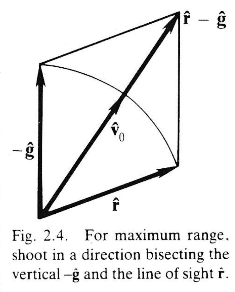
Fig. 2.4.
Substituting (2.11) in (2.8), one immediately finds the following expression for the maximum range:
\, r_{max} = \dfrac{ 2 {v_0}^2 }{g} \dfrac{ 1 }{ | \, \hat{\bold r} - \hat{\bold g} \, |^2 } = \dfrac{ 2 {v_0}^2 }{g} \dfrac{ 1 }{ 1 - \hat{\bold g} \cdot \hat{\bold r} }. \;\;\;\;\;\;\;\;\;\;\;\;\;\;\;\;\;\;\;\;\;\;\;\;\;\;\;\;\;\;\;\;\;\;\;\;\;\;\; (2.12)
We saw in Section 2-6 that this is an equation for a paraboloid of revolution; here, it expresses \, r_{max} \, as a function of the target direction \, \hat{\bold r} . As illustrated in Figure 2.5, the paraboloid is the envelope of all trajectories emanating from the origin with the same initial speed \, v_0 . Thus, only points under the paraboloid can be reached by a projectile.
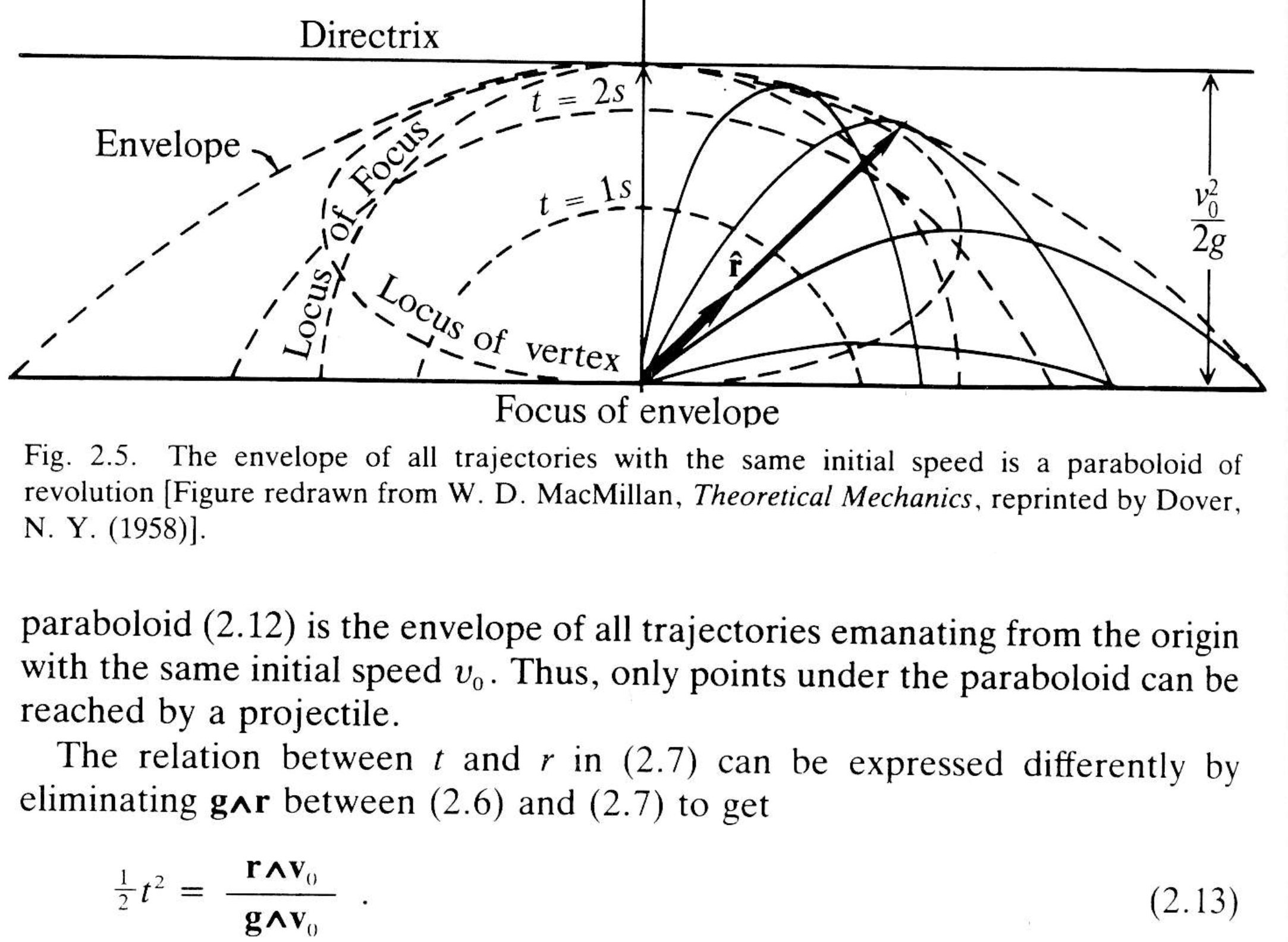
Fig. 2.5.
/// FORTSÄTT HÄR
/////// End of quote from Hestenes