This page is a sub-page of our page on Geometric Algebra.
///////
The sub-pages of this page are:
///////
Related KMR-pages:
• Clifford Algebra
• Geometric Algebra
• Complex Numbers
• Quaternions
///////
Other relevant sources of information:
• Rotor (at Wikipedia)
• Associative Composition Algebra (at Wikibooks)
• Quaternion (at Wikipedia)
• Rotor (at Wikipedia)
• Versor (at Wikipedia)
• Hyperbolic versor (at Wikipedia)
• Rotation formalisms in three dimensions (at Wikipedia)
///////
The interactive simulations on this page can be navigated with the Free Viewer
of the Graphing Calculator.
///////
\, \begin{bmatrix} \, x \, \\ \, y \, \\ \, z \, \end{bmatrix} \; \begin{bmatrix} -x \\ \; y \\ \; z \end{bmatrix} \; \begin{bmatrix} \; x \\ -y \\ \; z \end{bmatrix} \; \begin{bmatrix} \; x \\ \; y \\ -z \end{bmatrix} \; \begin{bmatrix} \; x \\ -y \\-z \end{bmatrix} \; \begin{bmatrix} -x \\ \; y \\ -z \end{bmatrix} \; \begin{bmatrix} -x \\ -y \\ \; z \end{bmatrix} \; \begin{bmatrix} -x \\ -y \\ -z \end{bmatrix}
///////

/////////////////////////////////////////////////////
Geometric numbers in Euclidean 3D-space:
\, R_{{eflect}\,i_{n}P_{lane}} (F_{orward}) \, \, R_{{eflect}\,i_{n}P_{lane}} (L_{eftward}) \, \, R_{{eflect}\,i_{n}P_{lane}} (U_{pward}) \,and the oppositely directed and equivalent reflection descriptions:
\, R_{{eflect}\,i_{n}P_{lane}} (B_{ackward}) \, = \, R_{{eflect}\,i_{n}P_{lane}} (F_{orward}) \, \, R_{{eflect}\,i_{n}P_{lane}} (R_{ightward}) \, = \, R_{{eflect}\,i_{n}P_{lane}} (L_{eftward}) \, \, R_{{eflect}\,i_{n}P_{lane}} (D_{ownward}) \, = \, R_{{eflect}\,i_{n}P_{lane}} (U_{pward}) \,///////
Dualisation:
\, (F_{orward} L_{eftward})^{\star} \, = \, (F_{orward} L_{eftward}) \, {(- \, F_{orward} L_{eftward} U_{pward})}^{-1} \, = \,
\, = \, - \, F_{orward} L_{eftward} (U_{pward})^{-1} (L_{eftward})^{-1} (F_{orward})^{-1} \, =
\, = \, - \, F_{orward} L_{eftward} D_{ownward} R_{ightward} B_{ackward} \, = \, F_{orward} L_{eftward} R_{ightward} D_{ownward} B_{ackward} \, =
\, = \, F_{orward} D_{ownward} B_{ackward} \, = \, - \, F_{orward} B_{ackward} D_{ownward} \, = \, - \, D_{ownward} \, = \, U_{pward}
\, (L_{eftward} U_{pward})^{\star} \, = \, (L_{eftward} U_{pward}) \, {(- F_{orward} L_{eftward} U_{pward})}^{-1} \, = \,
\, = \, - L_{eftward} U_{pward} (U_{pward})^{-1} (L_{eftward})^{-1} (F_{orward})^{-1} \, = \, - (F_{orward})^{-1} \, = \, - B_{ackward} \, = \, F_{orward}
\, (F_{orward} U_{pward})^{\star} \, = \, (F_{orward} U_{pward}) \, {(- \, F_{orward} L_{eftward} U_{pward})}^{-1} \, = \,
\, = \, - \, F_{orward} U_{pward} (U_{pward})^{-1} (L_{eftward})^{-1} (F_{orward})^{-1} \, =
\, = \, - \, F_{orward} R_{ightward} B_{ackward} \, = \, F_{orward} B_{ackward} R_{ightward} \, = \, R_{ightward} \, = \, - L_{eftward}
///////
Reflections in planes, lines and points
Three reflections in perpendicular planes produce a reflection
in the point of intersection of the three planes (= the origin):
A reflection in a line is equal to a halfturn around this line:
\, R_{{eflect}\,i_{n}L_{ine}} (a_{line}) \, = \, R_{otate(H{alf}T_{urn})\,a_{round}} (t_{{he}L_{ine}}) \,Two reflections in perpendicular planes produce a halfturn around their line of intersection :
\, R_{{eflect}\,i_{n}P_{lane}} (F_{orward}) R_{{eflect}\,i_{n}P_{lane}} (L_{eftward}) \, = \, R_{{eflect}\,i_{n}L_{ine}} (L_{ine}(F_{orward} L_{eftward})^{\star}) \, = \, R_{otate(H{alf}T_{urn})\,a_{round}} (L_{ine} (U_{pward})) \, \, R_{{eflect}\,i_{n}P_{lane}} (L_{eftward}) R_{{eflect}\,i_{n}P_{lane}} (U_{pward}) \, = \, R_{{eflect}\,i_{n}L_{ine}} (L_{ine}(L_{eftward} U_{pward})^{\star}) \, = \, R_{otate(H{alf}T_{urn})\,a_{round}} (L_{ine} (F_{orward})) \, \, R_{{eflect}\,i_{n}P_{lane}} (F_{orward}) R_{{eflect}\,i_{n}P_{lane}} (U_{pward}) \, = \, R_{{eflect}\,i_{n}L_{ine}} (L_{inje}(F_{orward} U_{pward})^{\star}) \, = \, R_{otate(H{alf}T_{urn})\,a_{round}} (L_{ine} (R_{ightward})) \,Moreover we have the relations:
\, R_{{eflect}\,i_{n}P_{lane}} (F_{orward}) R_{{eflect}\,i_{n}P_{lane}} (F_{orward}) \, = \, 1 \, \, R_{{eflect}\,i_{n}P_{lane}} (L_{eftward}) R_{{eflect}\,i_{n}P_{lane}} (L_{eftward}) \, = \, 1 \, \, R_{{eflect}\,i_{n}P_{lane}} (U_{pward}) R_{{eflect}\,i_{n}P_{lane}} (U_{pward}) \, = \, 1 \,///////
The algebraic structure of a planar reflection:
Theorem: Let \, P \, denote a plane in \, {\mathbb{R}}^3 \, with unit normal \, n .
In geometric algebra a reflection \, S_{P} \, in the plane \, P \, can be represented like this:
\, {\mathbb{R}}^3 \ni x \mapsto - \, n \, x \, n \, = \, \bar{x} = S_{P}(x) \in {\mathbb{R}}^3 .
Proof:
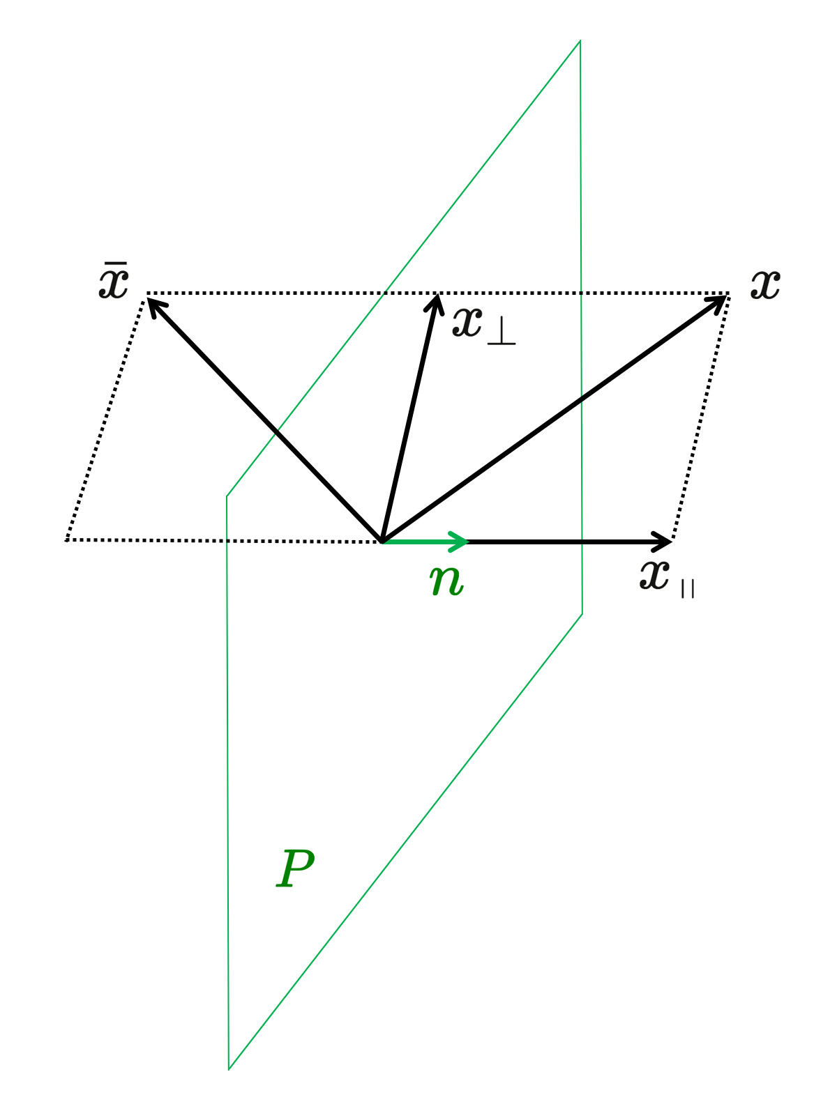
Reflection of the vector \, x \, in the plane \, P \, with unit normal \, n \, can be expressed as:
\, \bar{x} \, = \, - \, n \, x \, n \, = \, - \, n \, (x_{\, \shortparallel} + x_{\perp}) \, n \, = \, - \, n \, x_{\, \shortparallel} \, n - \, n \, x_{\perp} \, n \, = - \, n \, n \, x_{\, \shortparallel} + n \, n \, x_{\perp} \, = \, - \, x_{\, \shortparallel} + x_{\perp} \, = \, S_{P} (x) \,which finishes the proof.
Rotations
Two planar reflections make a rotation around their line of intersection.
General rotations can be performed by using versors.
Let the first and the second planar reflections have unit-normals \, m \, respectively \, n . Applying the reflection law twice, we get
\, \bar {\bar{x}} \, = \, - \, n \, ( - \, m \, x \, m ) \, n \, = \, n m \, x \, m n \, .
The algebraic and geometric structure of a versor:
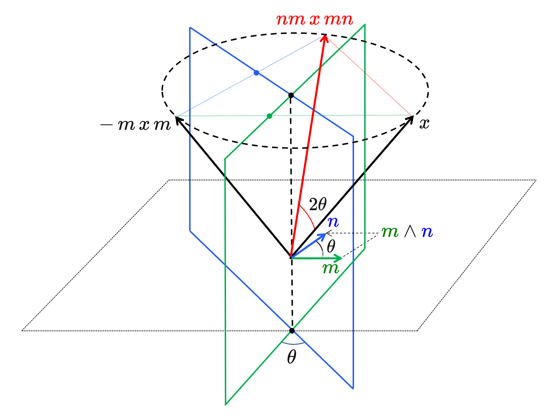
Notice that when \, \theta = \pi/2 \, the planes of reflection are perpendicular and we are back at the initial example. In this special case we have \, n m \, x \, m n \, = \, m n \, x \, n m \, and the corresponding half-turns are performed in opposite directions.
/////// Quoting Wikibooks Associative Composition Algebra / Division quaternions:
Lemma 1: If \, a \, and \, b \, are square roots of minus one and if \, a \perp b , then \, a \, b \, a \, = \, b \, .
Proof: \,\; 0 \, = \, a \, (a \, b + b \, a) \, = \, a^2 \, b + a \, b \, a \, = \, -b + a \, b \, a \, .
Lemma 2: Under the same hypothesis, \, a \perp a \, b \, and \, b \perp a \, b \, .
Proof (of \, a \perp a\, b) \, : \, a \, (a \, b) + (a \, b) \, a \, = \, -b + a \, b \, a \, = \, 0 \, .
Let \, u = e^{\, \theta \, \mathbf{r}} \, be a versor. There is a group action on \, \mathbb{H} \, determined by \, u \, :
Inner automorphism \, f \, : \, \mathbb{H} \, \ni \, q \, \mapsto \, u^{-1} q \, u \, \in \, \mathbb{H} \, .
Note that \, u \, commutes with all vectors in the plane \, \{\, x + y \, \mathbf{r} \, : \, x, y \, \in \, \mathbb{R} \, \} .
Select \, \mathbf{s} \, from the great circle on \, \mathbb{S}^2 \, that is perpendicular to \, \mathbf{r} .
Then \, \mathbf{r} \, \mathbf{s} \, \mathbf{r} \, = \, \mathbf{s} \, by the first lemma. Now compute \, f(\mathbf{s}) \, :
\;\;\;\;\;\;\;\;\;\;\;\; = \, ({\cos}^2 \theta - {\sin}^2 \theta) \, \mathbf{s} + (2\sin \theta \cos \theta) \, \mathbf{s} \, \mathbf{r} \, = \, \mathbf{s} \, \cos 2 \theta + \mathbf{s} \, \mathbf{r} \, \sin 2 \theta ,
which is a rotation by \, 2 \theta \, in the \, (\mathbf{s}, \mathbf{s} \, \mathbf{r}) \, plane.
This feature of \, \mathbb{H} , inner automorphism \, f \, producing rotation, has proven very useful.
/////// End of quote from Wikibooks
Two \, \theta -separated reflections give a \, 2 \theta -separating rotation:

In the case of the plane, the reflections are carried out in lines,
and in the case of 3D-space the reflections are carried out in planes.
///////
The action of a fixed versor on a rotating vector:
The film shows the red-tipped vector rotating around the grey circle. The red-tipped vector is first reflected in the horizontal yellow line (in the left window), and correspondingly, in the vertical yellow plane (in the right window), which results in the yellow vector.
This yellow vector is then reflected in the light-blue line (in the left window) and correspondingly, in the light-blue vertical plane (in the right window), which results in the light-blue vector.
Since the light-blue vector is related to the red-tipped vector by a constant rotation, the light-blue vector must follow the red-tipped vector – at a constant distance and at a constant angle – around the circular cone which has the \, z -axis as its axis of symmetry.
///////
The action of a variable versor on a fixed vector:
The variation of the versor is provided by the change of angle between the yellow line and the light-blue line (in the left window) – and hence by the corresponding change of angle between the yellow vertical plane and the light-blue vertical plane (in the right window).
///////
///////
Hyperbolic versors
/////// Quoting Wikipedia ( https://en.wikipedia.org/wiki/Versor#Hyperbolic_versor ):
A hyperbolic versor is a generalization of quaternionic versors to indefinite orthogonal groups, such as the Lorentz group. It is defined as a quantity of the form
\, \exp (a \, \mathbf{r}) \, = \, \cosh a + \mathbf{r} \, \sinh a \, , where \, | \, \mathbf{r} \, | \, = \, 1 \, .
Such elements arise in algebras of mixed signature, for example split-complex numbers or split-quaternions. It was the algebra of tessarines discovered by James Cockle in 1848 that first provided hyperbolic versors. In fact, James Cockle wrote the above equation (with \, \mathbf{j} \, in place of \, \mathbf{r} \, ) when he found that the tessarines included the new type of imaginary element.
This versor was used by Homersham Cox (1882/83) in relation to quaternion multiplication.[6][7] The primary exponent of hyperbolic versors was Alexander Macfarlane as he worked to shape quaternion theory to serve physical science.[8] He saw the modelling power of hyperbolic versors operating on the split-complex number plane, and in 1891 he introduced hyperbolic quaternions to extend the concept to 4-space. Problems in that algebra led to use of biquaternions after 1900. In a widely circulated review of 1899, Macfarlane said:
…the root of a quadratic equation may be versor in nature or scalar in nature. If it is versor in nature, then the part affected by the radical involves the axis perpendicular to the plane of reference, and this is so, whether the radical involves the square root of minus one or not. In the former case the versor is circular, in the latter hyperbolic.[9]
Today the concept of a one-parameter group subsumes the concepts of versor and hyperbolic versor as the terminology of Sophus Lie has replaced that of Hamilton and Macfarlane. In particular, for each \, \mathbf{r} \, such that \, \mathbf{r} \, \mathbf{r} = +1 \, or \, \mathbf{r} \, \mathbf{r} = -1 , the mapping \, a \, \mapsto \, \exp (a \, \mathbf{r}) \, takes the real line to a group of hyperbolic or ordinary versors. In the ordinary case, when \, \mathbf{r} \, and \, -\mathbf{r} \, are antipodes on a sphere, the one-parameter groups have the same points but are oppositely directed. In physics, this aspect of rotational symmetry is termed a doublet.
In 1911 Alfred Robb published his Optical Geometry of Motion in which he identified the parameter rapidity which specifies a change in frame of reference. This rapidity parameter corresponds to the real variable in a one-parameter group of hyperbolic versors. With the further development of special relativity the action of a hyperbolic versor came to be called a Lorentz boost.
/////// End of quote from Wikipedia (on hyperbolic versors)
Interlude:
1, e_1, e_2, e_3, e_1 e_2, e_1 e_3, e_2 e_3, e_1 e_2 e_3 ,
\, { \bold e}_1 { \bold e}_2 \, ,
Dualising the axis of rotation gives:
\, {\bold j} = {{\bold e}_3}^* = {\bold e}_3 {\bold I } = {\bold e}_3 {\bold e}_1 {\bold e}_2 {\bold e}_3 = {\bold e}_1 {\bold e}_2 { \bold e}_3 {\bold e}_3 = {\bold e}_1 {\bold e}_2 , .
<br>
e_0^2 = 1^2 = 1 \; ,
e_1^2 = 1 \; ,
(e_1 e_2)^2 = -1 \; ,
(e_1 e_2 e_3)^2 = -1 \; ,
(e_1 e_2 e_3 e_4)^2 = 1 \; ,
(e_1 e_2 e_3 e_4 e_5)^2 = 1 \; ,
(e_1 e_2 e_3 e_4 e_5 e_6)^2 = -1 \; ,
(e_1 e_2 e_3 e_4 e_5 e_6 e_7)^2 = -1 \, ,
\cdots \, .
The quaternions as the even subalgebra
of the clifford algebra \, C_l(e_1, e_2, e_3) \, over the real numbers \, \mathbb{R} .
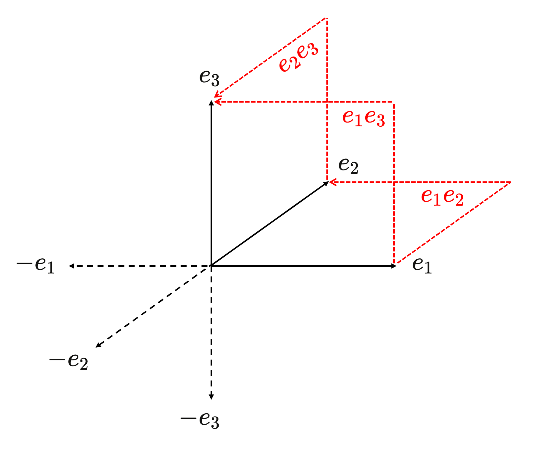
This diagram shows the 1-blades (unbroken black arrows) and the 2-blades (red, dotted, broken arrows) among the blades in the canonical basis for \, C_l(e_1, e_2, e_3) .
The negatives of the 1-blades are shown as dotted black arrows.
The 2-blades \, \textcolor {red} {e_1 e_2} \textcolor {black} {,} \textcolor {red} {e_2 e_3} \textcolor {black} {,} \textcolor {red} {e_1 e_3} \,
represent the directed area within the corresponding squares.
Hence we have for \, k \neq i \, : \, (e_i e_k)^2 = e_i e_k e_i e_k = - e_k e_i e_i e_k = - e_k e_k = -1 .
Addition rule for the even subalgebra of \, C_l(e_1, e_2, e_3) \, :
\, (\alpha \textcolor {red} 1 + \alpha_{12} \textcolor {red} {e_1 e_2} + \alpha_{23} \textcolor {red} {e_2 e_3} \, + \alpha_{13} \textcolor {red} {e_1 e_3}) \, +
\, + \, (\alpha' \textcolor {red} 1 +\alpha'_{12} \textcolor {red} {e_1 e_2} + \alpha'_{23} \textcolor {red} {e_2 e_3} + \alpha'_{13} \textcolor {red} {e_1 e_3}) \stackrel {\mathrm{def}}{=} \,
\stackrel {\mathrm{def}}{=} \, (\alpha + \alpha') \textcolor {red} 1 + (\alpha_{12} + \alpha'_{12}) \textcolor {red} {e_1 e_2} + (\alpha_{23} + \alpha'_{23}) \textcolor {red} {e_2 e_3} + (\alpha_{13} + \alpha'_{13}) \textcolor {red} {e_1 e_3} .
Multiplication table for the even subalgebra of \, C_l(e_1, e_2, e_3) \, :
\, \begin{matrix} * & ~ & \textcolor {red} 1 & \textcolor {red} {e_1 e_2} & \textcolor {red} {e_2 e_3} & \textcolor {red} {e_1 e_3} \\ & & & & & & \\ \textcolor {red} 1 & ~ & \textcolor {red} 1 & \textcolor {red} {e_1 e_2} & \textcolor {red} {e_2 e_3} & \textcolor {red} {e_1 e_3} \\ \textcolor {red} {e_1 e_2} & ~ & \textcolor {red} {e_1 e_2} & - \textcolor {red} 1 & \textcolor {red} {e_1 e_3} & - \textcolor {red} {e_2 e_3} \\ \textcolor {red} {e_2 e_3} & ~ & \textcolor {red} {e_2 e_3} & - \textcolor {red} {e_1 e_3} & - \textcolor {red} 1 & \textcolor {red} {e_1 e_2} \\ \textcolor {red} {e_1 e_3} & ~ & \textcolor {red} {e_1 e_3} & \textcolor {red} {e_2 e_3} & - \textcolor {red} {e_1 e_2} & - \textcolor {red} 1 \, \end{matrix} \,
Multiplication table for the quaternions:
///////
Substituting \, \bold 1 = \textcolor {red} {1} \, , \, \bold i = \textcolor {red} {e_1 e_2} \, , \, \bold j = \textcolor {red} {e_2 e_3} \, , \bold k = \textcolor {red} {e_1 e_3} \, and comparing the two multiplication tables, we see that they are identical, and therefore they represent the same mathematical structure.
///////
The 3D pseudoscalar
\, I \, = \, e_1 e_2 e_3 .
\, I^{-1} \, = \, e_3 e_2 e_1 .
\, I \, I^{-1} = e_1 e_2 e_3 e_3 e_2 e_1 \, = \, 1 .
\, I^{-1} \, I \, = \, e_3 e_2 e_1 e_1 e_2 e_3 \, = \, 1 .
\, I ^2 \, = \, e_1 e_2 e_3 e_1 e_2 e_3 \, = \, - e_2 e_1 e_3 e_1 e_2 e_3 \, = \, e_2 e_3 e_1 e_1 e_2 e_3 \, = \, e_2 e_3 e_2 e_3\, = \, - e_3 e_2 e_2 e_3 \, = \, - e_3 e_3 \, = \, -1 .
Duality
This page is a sub-page of our page on Geometric Algebra.
///////
The sub-pages of this page are:
///////
Related KMR-pages:
• Clifford Algebra
• Geometric Algebra
• Complex Numbers
• Quaternions
///////
Other relevant sources of information:
• Rotor (at Wikipedia)
• Associative Composition Algebra (at Wikibooks)
• Quaternion (at Wikipedia)
• Rotor (at Wikipedia)
• Versor (at Wikipedia)
• Hyperbolic versor (at Wikipedia)
• Rotation formalisms in three dimensions (at Wikipedia)
///////
The interactive simulations on this page can be navigated with the Free Viewer
of the Graphing Calculator.
///////
\, \begin{bmatrix} \, x \, \\ \, y \, \\ \, z \, \end{bmatrix} \; \begin{bmatrix} -x \\ \; y \\ \; z \end{bmatrix} \; \begin{bmatrix} \; x \\ -y \\ \; z \end{bmatrix} \; \begin{bmatrix} \; x \\ \; y \\ -z \end{bmatrix} \; \begin{bmatrix} \; x \\ -y \\-z \end{bmatrix} \; \begin{bmatrix} -x \\ \; y \\ -z \end{bmatrix} \; \begin{bmatrix} -x \\ -y \\ \; z \end{bmatrix} \; \begin{bmatrix} -x \\ -y \\ -z \end{bmatrix} .
///////
/////////////////////////////////////////////////////
Geometric numbers in Euclidean 3D-space:
\, R_{{eflect}\,i_{n}P_{lane}} (F_{orward}) \, \, R_{{eflect}\,i_{n}P_{lane}} (L_{eftward}) \, \, R_{{eflect}\,i_{n}P_{lane}} (U_{pward}) \,and the oppositely directed and equivalent reflection descriptions:
\, R_{{eflect}\,i_{n}P_{lane}} (B_{ackward}) \, = \, R_{{eflect}\,i_{n}P_{lane}} (F_{orward}) \, ,
\, R_{{eflect}\,i_{n}P_{lane}} (R_{ightward}) \, = \, R_{{eflect}\,i_{n}P_{lane}} (L_{eftward}) \, ,
\, R_{{eflect}\,i_{n}P_{lane}} (D_{ownward}) \, = \, R_{{eflect}\,i_{n}P_{lane}} (U_{pward}) \, .
///////
Dualisation:
\, (F_{orward} L_{eftward})^{\star} \, = \, (F_{orward} L_{eftward}) \, {(- \, F_{orward} L_{eftward} U_{pward})}^{-1} \, = \,
\, = \, - \, F_{orward} L_{eftward} (U_{pward})^{-1} (L_{eftward})^{-1} (F_{orward})^{-1} \, =
\, = \, - \, F_{orward} L_{eftward} D_{ownward} R_{ightward} B_{ackward} \, = \, F_{orward} L_{eftward} R_{ightward} D_{ownward} B_{ackward} \, =
\, = \, F_{orward} D_{ownward} B_{ackward} \, = \, - \, F_{orward} B_{ackward} D_{ownward} \, = \, - \, D_{ownward} \, = \, U_{pward} .
\, (L_{eftward} U_{pward})^{\star} \, = \, (L_{eftward} U_{pward}) \, {(- F_{orward} L_{eftward} U_{pward})}^{-1} \, = \,
\, = \, - L_{eftward} U_{pward} (U_{pward})^{-1} (L_{eftward})^{-1} (F_{orward})^{-1} \, = \, - (F_{orward})^{-1} \, = \, - B_{ackward} \, = \, F_{orward} .
\, (F_{orward} U_{pward})^{\star} \, = \, (F_{orward} U_{pward}) \, {(- \, F_{orward} L_{eftward} U_{pward})}^{-1} \, = \,
\, = \, - \, F_{orward} U_{pward} (U_{pward})^{-1} (L_{eftward})^{-1} (F_{orward})^{-1} \, =
\, = \, - \, F_{orward} R_{ightward} B_{ackward} \, = \, F_{orward} B_{ackward} R_{ightward} \, = \, R_{ightward} \, = \, - L_{eftward} .
///////
Reflections in planes, lines and points
Three reflections in perpendicular planes produce a reflection
in the point of intersection of the three planes (= the origin):
\, R_{{eflect}\,i_{n}P_{lane}} (F_{orward}) R_{{eflect}\,i_{n}P_{lane}} (L_{eftward}) R_{{eflect}\,i_{n}P_{lane}} (U_{pward}) \, = R_{{eflect}\,i_{n}P_{oint}} (O_{rigin}) \, = -1 \, .
A reflection in a line is equal to a halfturn around this line:
\, R_{{eflect}\,i_{n}L_{ine}} (a_{line}) \, = \, R_{otate(H{alf}T_{urn})\,a_{round}} (t_{{he}L_{ine}}) \, .
Two reflections in perpendicular planes produce a halfturn around their line of intersection :
\, R_{{eflect}\,i_{n}P_{lane}} (F_{orward}) R_{{eflect}\,i_{n}P_{lane}} (L_{eftward}) \, = \, R_{{eflect}\,i_{n}L_{ine}} (L_{ine}(F_{orward} L_{eftward})^{\star}) \, = \, R_{otate(H{alf}T_{urn})\,a_{round}} (L_{ine} (U_{pward})) \, .
\, R_{{eflect}\,i_{n}P_{lane}} (L_{eftward}) R_{{eflect}\,i_{n}P_{lane}} (U_{pward}) \, = \, R_{{eflect}\,i_{n}L_{ine}} (L_{ine}(L_{eftward} U_{pward})^{\star}) \, = \, R_{otate(H{alf}T_{urn})\,a_{round}} (L_{ine} (F_{orward})) \, .
\, R_{{eflect}\,i_{n}P_{lane}} (F_{orward}) R_{{eflect}\,i_{n}P_{lane}} (U_{pward}) \, = \, R_{{eflect}\,i_{n}L_{ine}} (L_{inje}(F_{orward} U_{pward})^{\star}) \, = \, R_{otate(H{alf}T_{urn})\,a_{round}} (L_{ine} (R_{ightward})) \, .
Moreover we have the relations:
\, R_{{eflect}\,i_{n}P_{lane}} (F_{orward}) R_{{eflect}\,i_{n}P_{lane}} (F_{orward}) \, = \, 1 \, ,
\, R_{{eflect}\,i_{n}P_{lane}} (L_{eftward}) R_{{eflect}\,i_{n}P_{lane}} (L_{eftward}) \, = \, 1 \, ,
\, R_{{eflect}\,i_{n}P_{lane}} (U_{pward}) R_{{eflect}\,i_{n}P_{lane}} (U_{pward}) \, = \, 1 \, .
///////
The algebraic structure of a planar reflection:
Theorem: Let \, P \, denote a plane in \, {\mathbb{R}}^3 \, with unit normal \, n .
In geometric algebra a reflection \, S_{P} \, in the plane \, P \, can be represented like this:
\, {\mathbb{R}}^3 \ni x \mapsto - \, n \, x \, n \, = \, \bar{x} = S_{P}(x) \in {\mathbb{R}}^3 .
Proof:
Reflection of the vector \, x \, in the plane \, P \, with unit normal \, n \, can be expressed as:
\, \bar{x} \, = \, - \, n \, x \, n \, = \, - \, n \, (x_{\, \shortparallel} + x_{\perp}) \, n \, = \, - \, n \, x_{\, \shortparallel} \, n - \, n \, x_{\perp} \, n \, = - \, n \, n \, x_{\, \shortparallel} + n \, n \, x_{\perp} \, = \, - \, x_{\, \shortparallel} + x_{\perp} \, = \, S_{P} (x) \,which finishes the proof.
Rotations
Two planar reflections make a rotation around their line of intersection.
General rotations can be performed by using versors.
Let the first and the second planar reflections have unit-normals \, m \, respectively \, n . Applying the reflection law twice, we get
\, \bar {\bar{x}} \, = \, - \, n \, ( - \, m \, x \, m ) \, n \, = \, n m \, x \, m n \,
The algebraic and geometric structure of a versor:
Notice that when \, \theta = \pi/2 \, the planes of reflection are perpendicular and we are back at the initial example. In this special case we have \, n m \, x \, m n \, = \, m n \, x \, n m \, and the corresponding half-turns are performed in opposite directions.
/////// Quoting Wikibooks Associative Composition Algebra / Division quaternions:
Lemma 1: If \, a \, and \, b \, are square roots of minus one and if \, a \perp b , then \, a \, b \, a \, = \, b \, .
Proof: \,\; 0 \, = \, a \, (a \, b + b \, a) \, = \, a^2 \, b + a \, b \, a \, = \, -b + a \, b \, a \, .
Lemma 2: Under the same hypothesis, \, a \perp a \, b \, and \, b \perp a \, b \, .
Proof (of \, a \perp a\, b) \, : \, a \, (a \, b) + (a \, b) \, a \, = \, -b + a \, b \, a \, = \, 0 \, .
Let \, u = e^{\, \theta \, \mathbf{r}} \, be a versor. There is a group action on \, \mathbb{H} \, determined by \, u \, :
Inner automorphism \, f \, : \, \mathbb{H} \, \ni \, q \, \mapsto \, u^{-1} q \, u \, \in \, \mathbb{H} \, .
Note that \, u \, commutes with all vectors in the plane \, \{\, x + y \, \mathbf{r} \, : \, x, y \, \in \, \mathbb{R} \, \} .
Select \, \mathbf{s} \, from the great circle on \, \mathbb{S}^2 \, that is perpendicular to \, \mathbf{r} .
Then \, \mathbf{r} \, \mathbf{s} \, \mathbf{r} \, = \, \mathbf{s} \, by the first lemma. Now compute \, f(\mathbf{s}) \, :
\;\;\;\;\;\;\;\;\;\;\;\; = \, ({\cos}^2 \theta - {\sin}^2 \theta) \, \mathbf{s} + (2\sin \theta \cos \theta) \, \mathbf{s} \, \mathbf{r} \, = \, \mathbf{s} \, \cos 2 \theta + \mathbf{s} \, \mathbf{r} \, \sin 2 \theta ,
which is a rotation by \, 2 \theta \, in the \, (\mathbf{s}, \mathbf{s} \, \mathbf{r}) \, plane.
This feature of \, \mathbb{H} , inner automorphism \, f \, producing rotation, has proven very useful.
/////// End of quote from Wikibooks
Two \, \theta -separated reflections give a \, 2 \theta -separating rotation:
In the case of the plane, the reflections are carried out in lines,
and in the case of 3D-space the reflections are carried out in planes.
///////
The action of a fixed versor on a rotating vector:
The film shows the red-tipped vector rotating around the grey circle. The red-tipped vector is first reflected in the horizontal yellow line (in the left window), and correspondingly, in the vertical yellow plane (in the right window), which results in the yellow vector.
This yellow vector is then reflected in the light-blue line (in the left window) and correspondingly, in the light-blue vertical plane (in the right window), which results in the light-blue vector.
Since the light-blue vector is related to the red-tipped vector by a constant rotation, the light-blue vector must follow the red-tipped vector – at a constant distance and at a constant angle – around the circular cone which has the \, z -axis as its axis of symmetry.
///////
The action of a variable versor on a fixed vector:
The variation of the versor is provided by the change of angle between the yellow line and the light-blue line (in the left window) – and hence by the corresponding change of angle between the yellow vertical plane and the light-blue vertical plane (in the right window).
///////
Hyperbolic versors
/////// Quoting Wikipedia ( https://en.wikipedia.org/wiki/Versor#Hyperbolic_versor ):
A hyperbolic versor is a generalization of quaternionic versors to indefinite orthogonal groups, such as the Lorentz group. It is defined as a quantity of the form
\, \exp (a \, \mathbf{r}) \, = \, \cosh a + \mathbf{r} \, \sinh a \, , where \, | \, \mathbf{r} \, | \, = \, 1 \, .
Such elements arise in algebras of mixed signature, for example split-complex numbers or split-quaternions. It was the algebra of tessarines discovered by James Cockle in 1848 that first provided hyperbolic versors. In fact, James Cockle wrote the above equation (with \, \mathbf{j} \, in place of \, \mathbf{r} \, ) when he found that the tessarines included a new type of imaginary element.
This versor was used by Homersham Cox (1882/83) in relation to quaternion multiplication.[6][7] The primary exponent of hyperbolic versors was Alexander Macfarlane as he worked to shape quaternion theory to serve physical science.[8] He saw the modelling power of hyperbolic versors operating on the split-complex number plane, and in 1891 he introduced hyperbolic quaternions to extend the concept to 4-space. Problems in that algebra led to use of biquaternions after 1900. In a widely circulated review of 1899, Macfarlane said:
…the root of a quadratic equation may be versor in nature or scalar in nature. If it is versor in nature, then the part affected by the radical involves the axis perpendicular to the plane of reference, and this is so, whether the radical involves the square root of minus one or not. In the former case the versor is circular, in the latter hyperbolic.[9]
Today the concept of a one-parameter group subsumes the concepts of versor and hyperbolic versor as the terminology of Sophus Lie has replaced that of Hamilton and Macfarlane. In particular, for each \, \mathbf{r} \, such that \, \mathbf{r} \, \mathbf{r} = +1 \, or \, \mathbf{r} \, \mathbf{r} = -1 , the mapping \, a \, \mapsto \, \exp (a \, \mathbf{r}) \, takes the real line to a group of hyperbolic or ordinary versors. In the ordinary case, when \, \mathbf{r} \, and \, -\mathbf{r} \, are antipodes on a sphere, the one-parameter groups have the same points but are oppositely directed. In physics, this aspect of rotational symmetry is termed a doublet.
In 1911 Alfred Robb published his Optical Geometry of Motion in which he identified the parameter rapidity which specifies a change in frame of reference. This rapidity parameter corresponds to the real variable in a one-parameter group of hyperbolic versors. With the further development of special relativity the action of a hyperbolic versor came to be called a Lorentz boost.
/////// End of quote from Wikipedia (on hyperbolic versors)
Interlude:
1, e_1, e_2, e_3, e_1 e_2, e_1 e_3, e_2 e_3, e_1 e_2 e_3 .
<br>
e_0^2 = 1^2 = 1 \; ,
e_1^2 = 1 \; ,
(e_1 e_2)^2 = -1 \; ,
(e_1 e_2 e_3)^2 = -1 \; ,
(e_1 e_2 e_3 e_4)^2 = 1 \; ,
(e_1 e_2 e_3 e_4 e_5)^2 = 1 \; ,
(e_1 e_2 e_3 e_4 e_5 e_6)^2 = -1 \; ,
(e_1 e_2 e_3 e_4 e_5 e_6 e_7)^2 = -1 \, ,
\cdots \, .
The quaternions as the even subalgebra
of the clifford algebra \, C_l(e_1, e_2, e_3) \, over the real numbers \, \mathbb{R} .
This diagram shows the 1-blades (unbroken black arrows) and the 2-blades (red, dotted, broken arrows) among the blades in the canonical basis for \, C_l(e_1, e_2, e_3) .
The negatives of the 1-blades are shown as dotted black arrows.
The 2-blades \, \textcolor {red} {e_1 e_2} \textcolor {black} {,} \textcolor {red} {e_2 e_3} \textcolor {black} {,} \textcolor {red} {e_1 e_3} \,
represent the directed area within the corresponding squares.
Hence we have for \, k \neq i \, : \, (e_i e_k)^2 = e_i e_k e_i e_k = - e_k e_i e_i e_k = - e_k e_k = -1 .
Addition rule for the even subalgebra of \, C_l(e_1, e_2, e_3) \, :
\, (\alpha \textcolor {red} 1 + \alpha_{12} \textcolor {red} {e_1 e_2} + \alpha_{23} \textcolor {red} {e_2 e_3} \, + \alpha_{13} \textcolor {red} {e_1 e_3}) \, +
\, + \, (\alpha' \textcolor {red} 1 +\alpha'_{12} \textcolor {red} {e_1 e_2} + \alpha'_{23} \textcolor {red} {e_2 e_3} + \alpha'_{13} \textcolor {red} {e_1 e_3}) \stackrel {\mathrm{def}}{=} \,
\stackrel {\mathrm{def}}{=} \, (\alpha + \alpha') \textcolor {red} 1 + (\alpha_{12} + \alpha'_{12}) \textcolor {red} {e_1 e_2} + (\alpha_{23} + \alpha'_{23}) \textcolor {red} {e_2 e_3} + (\alpha_{13} + \alpha'_{13}) \textcolor {red} {e_1 e_3} .
Multiplication table for the even subalgebra of \, C_l(e_1, e_2, e_3) \, :
\, \begin{matrix} * & ~ & \textcolor {red} 1 & \textcolor {red} {e_1 e_2} & \textcolor {red} {e_2 e_3} & \textcolor {red} {e_1 e_3} \\ & & & & & & \\ \textcolor {red} 1 & ~ & \textcolor {red} 1 & \textcolor {red} {e_1 e_2} & \textcolor {red} {e_2 e_3} & \textcolor {red} {e_1 e_3} \\ \textcolor {red} {e_1 e_2} & ~ & \textcolor {red} {e_1 e_2} & - \textcolor {red} 1 & \textcolor {red} {e_1 e_3} & - \textcolor {red} {e_2 e_3} \\ \textcolor {red} {e_2 e_3} & ~ & \textcolor {red} {e_2 e_3} & - \textcolor {red} {e_1 e_3} & - \textcolor {red} 1 & \textcolor {red} {e_1 e_2} \\ \textcolor {red} {e_1 e_3} & ~ & \textcolor {red} {e_1 e_3} & \textcolor {red} {e_2 e_3} & - \textcolor {red} {e_1 e_2} & - \textcolor {red} 1 \, \end{matrix} \, .
Multiplication table for the quaternions:
\, \begin{matrix} * & ~ & \bold 1 & \;\; \bold i & \;\; \bold j & \, \;\, \bold k \\ & & & & & & \\ \bold 1 & ~ & \bold 1 & \;\; \bold i & \;\; \bold j & \;\; \bold k \\ \bold i & ~ & \bold i & - \bold 1 & \;\; \bold k & - \bold j \\ \bold j & ~ & \bold j & - \bold k & - \bold 1 & \;\; \bold i \\ \bold k & ~ & \bold k & \;\; \bold j & - \bold i & - \bold 1 \, \end{matrix} \,///////
Substituting \, \bold 1 = \textcolor {red} {1} \, , \, \bold i = \textcolor {red} {e_1 e_2} \, , \, \bold j = \textcolor {red} {e_2 e_3} \, , \bold k = \textcolor {red} {e_1 e_3} \, and comparing the two multiplication tables, we see that they are identical, and therefore they represent the same mathematical structure.
///////
The 3D pseudoscalar
\, I \, = \, e_1 e_2 e_3 .
\, I^{-1} \, = \, e_3 e_2 e_1 .
\, I \, I^{-1} = e_1 e_2 e_3 e_3 e_2 e_1 \, = \, 1 .
\, I^{-1} \, I \, = \, e_3 e_2 e_1 e_1 e_2 e_3 \, = \, 1 .
\, I ^2 \, = \, e_1 e_2 e_3 e_1 e_2 e_3 \, = \, - e_2 e_1 e_3 e_1 e_2 e_3 \, = \, e_2 e_3 e_1 e_1 e_2 e_3 \, = \, e_2 e_3 e_2 e_3\, = \, - e_3 e_2 e_2 e_3 \, = \, - e_3 e_3 \, = \, -1 .
Duality
This page is a sub-page of our page on Geometric Algebra.
///////
The sub-pages of this page are:
///////
Related KMR-pages:
• Clifford Algebra
• Geometric Algebra
• Complex Numbers
• Quaternions
///////
Other relevant sources of information:
• Rotor (at Wikipedia)
• Associative Composition Algebra (at Wikibooks)
• Quaternion (at Wikipedia)
• Rotor (at Wikipedia)
• Versor (at Wikipedia)
• Hyperbolic versor (at Wikipedia)
• Rotation formalisms in three dimensions (at Wikipedia)
///////
The interactive simulations on this page can be navigated with the Free Viewer
of the Graphing Calculator.
///////
\, \begin{bmatrix} \, x \, \\ \, y \, \\ \, z \, \end{bmatrix} \; \begin{bmatrix} -x \\ \; y \\ \; z \end{bmatrix} \; \begin{bmatrix} \; x \\ -y \\ \; z \end{bmatrix} \; \begin{bmatrix} \; x \\ \; y \\ -z \end{bmatrix} \; \begin{bmatrix} \; x \\ -y \\-z \end{bmatrix} \; \begin{bmatrix} -x \\ \; y \\ -z \end{bmatrix} \; \begin{bmatrix} -x \\ -y \\ \; z \end{bmatrix} \; \begin{bmatrix} -x \\ -y \\ -z \end{bmatrix}
///////
/////////////////////////////////////////////////////
Geometric numbers in Euclidean 3D-space:
\, R_{{eflect}\,i_{n}P_{lane}} (F_{orward}) \, \, R_{{eflect}\,i_{n}P_{lane}} (L_{eftward}) \, \, R_{{eflect}\,i_{n}P_{lane}} (U_{pward}) \,and the oppositely directed and equivalent reflection descriptions:
\, R_{{eflect}\,i_{n}P_{lane}} (B_{ackward}) \, = \, R_{{eflect}\,i_{n}P_{lane}} (F_{orward}) \, \, R_{{eflect}\,i_{n}P_{lane}} (R_{ightward}) \, = \, R_{{eflect}\,i_{n}P_{lane}} (L_{eftward}) \, \, R_{{eflect}\,i_{n}P_{lane}} (D_{ownward}) \, = \, R_{{eflect}\,i_{n}P_{lane}} (U_{pward}) \,///////
Dualisation:
\, (F_{orward} L_{eftward})^{\star} \, = \, (F_{orward} L_{eftward}) \, {(- \, F_{orward} L_{eftward} U_{pward})}^{-1} \, = \,
\, = \, - \, F_{orward} L_{eftward} (U_{pward})^{-1} (L_{eftward})^{-1} (F_{orward})^{-1} \, =
\, = \, - \, F_{orward} L_{eftward} D_{ownward} R_{ightward} B_{ackward} \, = \, F_{orward} L_{eftward} R_{ightward} D_{ownward} B_{ackward} \, =
\, = \, F_{orward} D_{ownward} B_{ackward} \, = \, - \, F_{orward} B_{ackward} D_{ownward} \, = \, - \, D_{ownward} \, = \, U_{pward}
\, (L_{eftward} U_{pward})^{\star} \, = \, (L_{eftward} U_{pward}) \, {(- F_{orward} L_{eftward} U_{pward})}^{-1} \, = \,
\, = \, - L_{eftward} U_{pward} (U_{pward})^{-1} (L_{eftward})^{-1} (F_{orward})^{-1} \, = \, - (F_{orward})^{-1} \, = \, - B_{ackward} \, = \, F_{orward}
\, (F_{orward} U_{pward})^{\star} \, = \, (F_{orward} U_{pward}) \, {(- \, F_{orward} L_{eftward} U_{pward})}^{-1} \, = \,
\, = \, - \, F_{orward} U_{pward} (U_{pward})^{-1} (L_{eftward})^{-1} (F_{orward})^{-1} \, =
\, = \, - \, F_{orward} R_{ightward} B_{ackward} \, = \, F_{orward} B_{ackward} R_{ightward} \, = \, R_{ightward} \, = \, - L_{eftward}
///////
Reflections in planes, lines and points
Three reflections in perpendicular planes produce a reflection
in the point of intersection of the three planes (= the origin):
A reflection in a line is equal to a halfturn around this line:
\, R_{{eflect}\,i_{n}L_{ine}} (a_{line}) \, = \, R_{otate(H{alf}T_{urn})\,a_{round}} (t_{{he}L_{ine}}) \,Two reflections in perpendicular planes produce a halfturn around their line of intersection :
\, R_{{eflect}\,i_{n}P_{lane}} (F_{orward}) R_{{eflect}\,i_{n}P_{lane}} (L_{eftward}) \, = \, R_{{eflect}\,i_{n}L_{ine}} (L_{ine}(F_{orward} L_{eftward})^{\star}) \, = \, R_{otate(H{alf}T_{urn})\,a_{round}} (L_{ine} (U_{pward})) \, \, R_{{eflect}\,i_{n}P_{lane}} (L_{eftward}) R_{{eflect}\,i_{n}P_{lane}} (U_{pward}) \, = \, R_{{eflect}\,i_{n}L_{ine}} (L_{ine}(L_{eftward} U_{pward})^{\star}) \, = \, R_{otate(H{alf}T_{urn})\,a_{round}} (L_{ine} (F_{orward})) \, \, R_{{eflect}\,i_{n}P_{lane}} (F_{orward}) R_{{eflect}\,i_{n}P_{lane}} (U_{pward}) \, = \, R_{{eflect}\,i_{n}L_{ine}} (L_{inje}(F_{orward} U_{pward})^{\star}) \, = \, R_{otate(H{alf}T_{urn})\,a_{round}} (L_{ine} (R_{ightward})) \,Moreover we have the relations:
\, R_{{eflect}\,i_{n}P_{lane}} (F_{orward}) R_{{eflect}\,i_{n}P_{lane}} (F_{orward}) \, = \, 1 \, \, R_{{eflect}\,i_{n}P_{lane}} (L_{eftward}) R_{{eflect}\,i_{n}P_{lane}} (L_{eftward}) \, = \, 1 \, \, R_{{eflect}\,i_{n}P_{lane}} (U_{pward}) R_{{eflect}\,i_{n}P_{lane}} (U_{pward}) \, = \, 1 \,///////
The algebraic structure of a planar reflection:
Theorem: Let \, P \, denote a plane in \, {\mathbb{R}}^3 \, with unit normal \, n .
In geometric algebra a reflection \, S_{P} \, in the plane \, P \, can be represented like this:
\, {\mathbb{R}}^3 \ni x \mapsto - \, n \, x \, n \, = \, \bar{x} = S_{P}(x) \in {\mathbb{R}}^3 .
Proof:
Reflection of the vector \, x \, in the plane \, P \, with unit normal \, n \, can be expressed as:
\, \bar{x} \, = \, - \, n \, x \, n \, = \, - \, n \, (x_{\, \shortparallel} + x_{\perp}) \, n \, = \, - \, n \, x_{\, \shortparallel} \, n - \, n \, x_{\perp} \, n \, = - \, n \, n \, x_{\, \shortparallel} + n \, n \, x_{\perp} \, = \, - \, x_{\, \shortparallel} + x_{\perp} \, = \, S_{P} (x) \,which finishes the proof.
Rotations
Two planar reflections make a rotation around their line of intersection.
General rotations can be performed by using versors.
Let the first and the second planar reflections have unit-normals \, m \, respectively \, n . Applying the reflection law twice, we get
\, \bar {\bar{x}} \, = \, - \, n \, ( - \, m \, x \, m ) \, n \, = \, n m \, x \, m n \,
The algebraic and geometric structure of a versor:
Notice that when \, \theta = \pi/2 \, the planes of reflection are perpendicular and we are back at the initial example. In this special case we have \, n m \, x \, m n \, = \, m n \, x \, n m \, and the corresponding half-turns are performed in opposite directions.
/////// Quoting Wikibooks Associative Composition Algebra / Division quaternions:
Lemma 1: If \, a \, and \, b \, are square roots of minus one and if \, a \perp b , then \, a \, b \, a \, = \, b \, .
Proof: \,\; 0 \, = \, a \, (a \, b + b \, a) \, = \, a^2 \, b + a \, b \, a \, = \, -b + a \, b \, a \, .
Lemma 2: Under the same hypothesis, \, a \perp a \, b \, and \, b \perp a \, b \, .
Proof (of \, a \perp a\, b) \, : \, a \, (a \, b) + (a \, b) \, a \, = \, -b + a \, b \, a \, = \, 0 \, .
Let \, u = e^{\, \theta \, \mathbf{r}} \, be a versor. There is a group action on \, \mathbb{H} \, determined by \, u \, :
Inner automorphism \, f \, : \, \mathbb{H} \, \ni \, q \, \mapsto \, u^{-1} q \, u \, \in \, \mathbb{H} \, .
Note that \, u \, commutes with all vectors in the plane \, \{\, x + y \, \mathbf{r} \, : \, x, y \, \in \, \mathbb{R} \, \} .
Select \, \mathbf{s} \, from the great circle on \, \mathbb{S}^2 \, that is perpendicular to \, \mathbf{r} .
Then \, \mathbf{r} \, \mathbf{s} \, \mathbf{r} \, = \, \mathbf{s} \, by the first lemma. Now compute \, f(\mathbf{s}) \, :
\;\;\;\;\;\;\;\;\;\;\;\; = \, ({\cos}^2 \theta - {\sin}^2 \theta) \, \mathbf{s} + (2\sin \theta \cos \theta) \, \mathbf{s} \, \mathbf{r} \, = \, \mathbf{s} \, \cos 2 \theta + \mathbf{s} \, \mathbf{r} \, \sin 2 \theta ,
which is a rotation by \, 2 \theta \, in the \, (\mathbf{s}, \mathbf{s} \, \mathbf{r}) \, plane.
This feature of \, \mathbb{H} , inner automorphism \, f \, producing rotation, has proven very useful.
/////// End of quote from Wikibooks
Two \, \theta -separated reflections give a \, 2 \theta -separating rotation:
In the case of the plane, the reflections are carried out in lines,
and in the case of 3D-space the reflections are carried out in planes.
///////
The action of a fixed versor on a rotating vector:
The film shows the red-tipped vector rotating around the grey circle. The red-tipped vector is first reflected in the horizontal yellow line (in the left window), and correspondingly, in the vertical yellow plane (in the right window), which results in the yellow vector.
This yellow vector is then reflected in the light-blue line (in the left window) and correspondingly, in the light-blue vertical plane (in the right window), which results in the light-blue vector.
Since the light-blue vector is related to the red-tipped vector by a constant rotation, the light-blue vector must follow the red-tipped vector – at a constant distance and at a constant angle – around the circular cone which has the \, z -axis as its axis of symmetry.
///////
The action of a variable versor on a fixed vector:
The variation of the versor is provided by the change of angle between the yellow line and the light-blue line (in the left window) – and hence by the corresponding change of angle between the yellow vertical plane and the light-blue vertical plane (in the right window).
///////
///////
Hyperbolic versors
/////// Quoting Wikipedia ( https://en.wikipedia.org/wiki/Versor#Hyperbolic_versor ):
A hyperbolic versor is a generalization of quaternionic versors to indefinite orthogonal groups, such as the Lorentz group. It is defined as a quantity of the form
\, \exp (a \, \mathbf{r}) \, = \, \cosh a + \mathbf{r} \, \sinh a \, , where \, | \, \mathbf{r} \, | \, = \, 1 \, .
Such elements arise in algebras of mixed signature, for example split-complex numbers or split-quaternions. It was the algebra of tessarines discovered by James Cockle in 1848 that first provided hyperbolic versors. In fact, James Cockle wrote the above equation (with \, \mathbf{j} \, in place of \, \mathbf{r} \, ) when he found that the tessarines included the new type of imaginary element.
This versor was used by Homersham Cox (1882/83) in relation to quaternion multiplication.[6][7] The primary exponent of hyperbolic versors was Alexander Macfarlane as he worked to shape quaternion theory to serve physical science.[8] He saw the modelling power of hyperbolic versors operating on the split-complex number plane, and in 1891 he introduced hyperbolic quaternions to extend the concept to 4-space. Problems in that algebra led to use of biquaternions after 1900. In a widely circulated review of 1899, Macfarlane said:
…the root of a quadratic equation may be versor in nature or scalar in nature. If it is versor in nature, then the part affected by the radical involves the axis perpendicular to the plane of reference, and this is so, whether the radical involves the square root of minus one or not. In the former case the versor is circular, in the latter hyperbolic.[9]
Today the concept of a one-parameter group subsumes the concepts of versor and hyperbolic versor as the terminology of Sophus Lie has replaced that of Hamilton and Macfarlane. In particular, for each \, \mathbf{r} \, such that \, \mathbf{r} \, \mathbf{r} = +1 \, or \, \mathbf{r} \, \mathbf{r} = -1 , the mapping \, a \, \mapsto \, \exp (a \, \mathbf{r}) \, takes the real line to a group of hyperbolic or ordinary versors. In the ordinary case, when \, \mathbf{r} \, and \, -\mathbf{r} \, are antipodes on a sphere, the one-parameter groups have the same points but are oppositely directed. In physics, this aspect of rotational symmetry is termed a doublet.
In 1911 Alfred Robb published his Optical Geometry of Motion in which he identified the parameter rapidity which specifies a change in frame of reference. This rapidity parameter corresponds to the real variable in a one-parameter group of hyperbolic versors. With the further development of special relativity the action of a hyperbolic versor came to be called a Lorentz boost.
/////// End of quote from Wikipedia (on hyperbolic versors)
Interlude:
<br>
e_0^2 = 1^2 = 1 \; ,
e_1^2 = 1 \; ,
(e_1 e_2)^2 = -1 \; ,
(e_1 e_2 e_3)^2 = -1 \; ,
(e_1 e_2 e_3 e_4)^2 = 1 \; ,
(e_1 e_2 e_3 e_4 e_5)^2 = 1 \; ,
(e_1 e_2 e_3 e_4 e_5 e_6)^2 = -1 \; ,
(e_1 e_2 e_3 e_4 e_5 e_6 e_7)^2 = -1 \, ,
\cdots \, .
The quaternions as the even subalgebra
of the clifford algebra \, C_l(e_1, e_2, e_3) \, over the real numbers \, \mathbb{R} .
This diagram shows the 1-blades (unbroken black arrows) and the 2-blades (red, dotted, broken arrows) among the blades in the canonical basis for \, C_l(e_1, e_2, e_3) .
The negatives of the 1-blades are shown as dotted black arrows.
The 2-blades \, \textcolor {red} {e_1 e_2} \textcolor {black} {,} \textcolor {red} {e_2 e_3} \textcolor {black} {,} \textcolor {red} {e_1 e_3} \,
represent the directed area within the corresponding squares.
Hence we have for \, k \neq i \, : \, (e_i e_k)^2 = e_i e_k e_i e_k = - e_k e_i e_i e_k = - e_k e_k = -1
Addition rule for the even subalgebra of \, C_l(e_1, e_2, e_3) \, :
\, (\alpha \textcolor {red} 1 + \alpha_{12} \textcolor {red} {e_1 e_2} + \alpha_{23} \textcolor {red} {e_2 e_3} \, + \alpha_{13} \textcolor {red} {e_1 e_3}) \, +
\, + \, (\alpha' \textcolor {red} 1 +\alpha'_{12} \textcolor {red} {e_1 e_2} + \alpha'_{23} \textcolor {red} {e_2 e_3} + \alpha'_{13} \textcolor {red} {e_1 e_3}) \stackrel {\mathrm{def}}{=} \,
\stackrel {\mathrm{def}}{=} \, (\alpha + \alpha') \textcolor {red} 1 + (\alpha_{12} + \alpha'_{12}) \textcolor {red} {e_1 e_2} + (\alpha_{23} + \alpha'_{23}) \textcolor {red} {e_2 e_3} + (\alpha_{13} + \alpha'_{13}) \textcolor {red} {e_1 e_3} .
Multiplication table for the even subalgebra of \, C_l(e_1, e_2, e_3) \, :
\, \begin{matrix} * & ~ & \textcolor {red} 1 & \textcolor {red} {e_1 e_2} & \textcolor {red} {e_2 e_3} & \textcolor {red} {e_1 e_3} \\ & & & & & & \\ \textcolor {red} 1 & ~ & \textcolor {red} 1 & \textcolor {red} {e_1 e_2} & \textcolor {red} {e_2 e_3} & \textcolor {red} {e_1 e_3} \\ \textcolor {red} {e_1 e_2} & ~ & \textcolor {red} {e_1 e_2} & - \textcolor {red} 1 & \textcolor {red} {e_1 e_3} & - \textcolor {red} {e_2 e_3} \\ \textcolor {red} {e_2 e_3} & ~ & \textcolor {red} {e_2 e_3} & - \textcolor {red} {e_1 e_3} & - \textcolor {red} 1 & \textcolor {red} {e_1 e_2} \\ \textcolor {red} {e_1 e_3} & ~ & \textcolor {red} {e_1 e_3} & \textcolor {red} {e_2 e_3} & - \textcolor {red} {e_1 e_2} & - \textcolor {red} 1 \, \end{matrix} \,
Multiplication table for the quaternions:
///////
Substituting \, \bold 1 = \textcolor {red} {1} \, , \, \bold i = \textcolor {red} {e_1 e_2} \, , \, \bold j = \textcolor {red} {e_2 e_3} \, , \bold k = \textcolor {red} {e_1 e_3} \, and comparing the two multiplication tables, we see that they are identical, and therefore they represent the same mathematical structure.
///////
The 3D pseudoscalar :
I = e_1 e_2 e_3 .
I^{-1} = e_3 e_2 e_1 .
I \, I^{-1} = e_1 e_2 e_3 e_3 e_2 e_1 = 1 .
I^{-1} I = \, e_3 e_2 e_1 e_1 e_2 e_3 = 1 .
I ^2 = e_1 e_2 e_3 e_1 e_2 e_3 = - e_2 e_1 e_3 e_1 e_2 e_3 = e_2 e_3 e_1 e_1 e_2 e_3 = e_2 e_3 e_2 e_3= - e_3 e_2 e_2 e_3 \, = \, - e_3 e_3 = -1 .
Duality of basis 1-blades:
= - e_3 e_1 e_1 e_2 = - e_3 e_2 = e_2 e_3 = e_2 \wedge e_3 .
{e_2}^* = - e_2 I^{-1} = - e_2 e_3 e_2 e_1 = e_3 e_2 e_2 e_1 = e_3 e_1 = e_3 \wedge e_1.
\, {e_3}^*= - e_3 I^{-1} = - e_3 e_3 e_2 e_1 = - e_2 e_1 = e_1 e_2 = e_1 \wedge e_2 .
Checking thay duality is equal to complementarity to I under the geometric product :
e_1 {e_1}^* = e_1 e_2 e_3 = I .
e_2 {e_2}^* = e_2 e_3 e_1 = - e_2 e_1 e_3 = e_1 e_2 e_3 = I .
e_3 {e_3}^* = e_3 e_1 e_2 = - e_1 e_3 e_2 = e_1 e_2 e_3 = I .
Duality of general 1-vectors :
a = a_1 e_1 + a_2 e_2 + a_3 e_3 .
a^*= (a_1 e_1 + a_2 e_2 + a_3 e_3)^*= a_1 e_2 e_3 + a_2 e_3 e_1 + a_3 e_1 e_2 .
b = b_1 e_1 + b_2 e_2 + b_3 e_3 .
b^*= (b_1 e_1 + b_2 e_2 + b_3 e_3)^*= b_1 e_2 e_3 + b_2 e_3 e_1 + b_3 e_1 e_2 .
Outer product of 1-vectors a and b :
a{\wedge}b = (a_1 e_1 + a_2 e_2 + a_3 e_3) \wedge (b_1 e_1 + b_2 e_2 + b_3 e_3) = a_1 b_2 e_1 e_2 + a_1 b_3 e_1 e_3 + a_2 b_1 e_2 e_1 + a_2 b_3 e_2 e_3 + a_3 b_1 e_3 e_1 + a_3 b_2 e_3 e_2 = (a_1 b_2 - a_2 b_1) e_1 e_2 + (a_1 b_3 - a_3 b_1) e_1 e_3 + (a_2 b_3 - a_3 b_2) e_2 e_3 .
Hence we have :
a{\wedge}b = (a_1 b_2 - a_2 b_1) {e_1}^* - (a_1 b_3 - a_3 b_1) {e_2}^* + (a_2 b_3 - a_3 b_2) {e_3}^* .
Comparison with the cross product of a and b :
a{\times}b = (a_1 b_2 - a_2 b_1) e_1 - (a_1 b_3 - a_3 b_1) e_2 + (a_2 b_3 - a_3 b_2) e_3 .
What are quaternions, and how do you visualize them? A story of four dimensions.
(Steven Strogatz on YouTube):
///////
Howdy! This is my first visit to your blog! We are a collection of volunteers and starting a new project in a community in the same niche. Your blog provided us useful information to work on. You have done a marvellous job!