This page is a sub-page of our page on Clifford Algebra.
///////
Related KMR pages:
///////
Other relevant sources of information:
• Combinatorial Aspects of Clifford Algebra, by Lars Svensson and Ambjörn Naeve (2002), presented at the International Workshop on Applications of Geometric Algebra, Cambridge, 5-6 Sept. 2002.
Svensson and Naeve (2002): Combinatorial aspects of Clifford Algebra
Abstract
In this paper we focus on some combinatorial aspects of Clifford algebra and show how this algebra allows combinatorial theorems – like e.g., Sperner’s lemma – to be “built into the algebraic background,” and become part of the structure of the algebra itself. We also give an example of how cumbersome combinatorial proofs can be “mechanized” and carried out in a purely computational manner.
Introduction
In his monumental and groundbreaking Ausdehnungslehre from 1844, Hermann Grassmann set out to build an “algebra for everything” – an algebra which he illustrated by various geometric examples. Being both far ahead of his time and on the outside of the academic mathematical community, Grassmann’s ideas received little attention during his own lifetime. However, during the last years of Grassmann’s life (late 1870s), his ideas were taken up by William Kingdon Clifford, who developed the algebra that today bears his name.
In more recent times, mathematicians and physicists – notably Marcel Riesz, Gian-Carlo Rota, and David Hestenes – have rediscovered and continued this development. Hestenes has focused on the geometric aspects of Clifford algebra – introducing the synonymous term geometric algebra – and shown how it provides a powerful geometric language that serves as a bridge between mathematics and physics.
In this paper we aim to connect with Grassmann’s original ideas and follow Rota by focusing on the purely combinatorial aspects of Clifford algebra.
Some notation and background
Since we are only interested in combinatorial and algebraic aspects of Clifford algebra, we will allow our scalars to lie in an arbitrary commutative ring \, \mathcal {R} \, with unit element. We will also take a slightly different point of view regarding the Clifford algebra and its interpretations.
Let \, E \, be a finite set which is totally ordered, i.e., \, E = \{e_1, \ldots, e_n\} \, where \, e_1 < e_2 < \ldots < e_n . We will identify the \, k -base-blades e_{n_1} e_{n_2} \ldots e_{n_k}, where \, e_1 < e_2 < \ldots < e_k \leq n, with the \, k -subsets \, \{e_{n_1}, \ldots, x_{e_k}\} \subseteq E \, and we will denote the pseudoscalar \, e_1 e_2 \ldots e_n \, by \, E \, (by an unproblematic change of context). Moreover, the ring unit \, 1 \, is identified with the empty set \, \emptyset .
We will view the Clifford algebra \, C_l(E) \, as the free \mathcal {R} -module
generated by the power-set \, \wp(E) \, of all subsets of \, E \, , i.e.,
C_l(E) = {\oplus \atop {e \in \wp(E) } } \mathcal {R} .
Note that if \, E \rightarrow E' \, is a bijection, then \, C_l(E) \, is isomorphic to \, C_l(E') . We will always assume that \, e^2 = 1, \forall e \in E . The set of \, k -vectors is denoted by {C_l}^k(E).
We observe that every bilinear map \, C_l(E) \times C_l(E) \longrightarrow C_l(E) \, is uniquely determined by its values on \, \wp(E) \times \wp(E) .
============
\, E = \{e_1, \ldots, e_n\} \, where \, e_1 < e_2 < \ldots < e_n .
{ \, e_1 \, e_2 \, e_3 \, e_4 \, e_5 \, e_6 \, e_7 \, e_8 \; e_9 \; e_{10} \, e_{11} \, e_{12} \, e_{13} \, e_{14} \, e_{15} \, e_{16} \, e_{17} \, e_{18} \, e_{19} \, e_{20} \, }///////
Other relevant sources of information:
• Combinatorial Aspects of Clifford Algebra, by Lars Svensson and Ambjörn Naeve (2002), presented at the International Workshop on Applications of Geometric Algebra, Cambridge, 5-6 Sept. 2002.
Svensson and Naeve (2002): Combinatorial aspects of Clifford Algebra
Abstract
In this paper we focus on some combinatorial aspects of Clifford algebra and show how this algebra allows combinatorial theorems – like e.g., Sperner’s lemma – to be “built into the algebraic background,” and become part of the structure of the algebra itself. We also give an example of how cumbersome combinatorial proofs can be “mechanized” and carried out in a purely computational manner.
Introduction
In his monumental and groundbreaking Ausdehnungslehre from 1844, Hermann Grassmann set out to build an “algebra for everything” – an algebra which he illustrated by various geometric examples. Being both far ahead of his time and on the outside of the academic mathematical community, Grassmann’s ideas received little attention during his own lifetime. However, during the last years of Grassmann’s life (late 1870s), his ideas were taken up by William Kingdon Clifford, who developed the algebra that today bears his name.
In more recent times, mathematicians and physicists – notably Marcel Riesz, Gian-Carlo Rota, and David Hestenes – have rediscovered and continued this development. Hestenes has focused on the geometric aspects of Clifford algebra – introducing the synonymous term geometric algebra – and shown how it provides a powerful geometric language that serves as a bridge between mathematics and physics.
In this paper we aim to connect with Grassmann’s original ideas and follow Rota by focusing on the purely combinatorial aspects of Clifford algebra.
Some notation and background
Since we are only interested in combinatorial and algebraic aspects of Clifford algebra, we will allow our scalars to lie in an arbitrary commutative ring \, \mathcal {R} \, with unit element. We will also take a slightly different point of view regarding the Clifford algebra and its interpretations.
Let \, E \, be a finite set which is totally ordered, i.e., \, E = \{e_1, \ldots, e_n\} \, where \, e_1 < e_2 < \ldots < e_n . We will identify the \, k -base-blades e_{n_1} e_{n_2} \ldots e_{n_k}, where \, e_1 < e_2 < \ldots < e_k \leq n, with the \, k -subsets \, \{e_{n_1}, \ldots, x_{e_k}\} \subseteq E \, and we will denote the pseudoscalar \, e_1 e_2 \ldots e_n \, by \, E \, (by an unproblematic change of context). Moreover, the ring unit \, 1 \, is identified with the empty set \, \emptyset .
We will view the Clifford algebra \, C_l(E) \, as the free \mathcal {R} -module
generated by the power-set \, \wp(E) \, of all subsets of \, E \, , i.e.,
C_l(E) = {\oplus \atop {e \in \wp(E) } } \mathcal {R} .
Note that if \, E \rightarrow E' \, is a bijection, then \, C_l(E) \, is isomorphic to \, C_l(E') . We will always assume that \, e^2 = 1, \forall e \in E . The set of \, k -vectors is denoted by {C_l}^k(E).
We observe that every bilinear map \, C_l(E) \times C_l(E) \longrightarrow C_l(E) \, is uniquely determined by its values on \, \wp(E) \times \wp(E) .
============
NOTATION: If \, P \, is a proposition, we will use \, (P) \, to denote \, 1 \, or \, 0 \,
\;\;\;\;\;\;\;\;\;\;\;\;\;\;\;\; depending on whether \, P \, is true or false.
Let \, A,B \in \wp(E) . The following definitions will be used:
Geometric product: \, A \, B = \epsilon \, A \, \Delta \, B, \,
where \, \epsilon = \pm 1 \, and \, \Delta \, is symmetric difference.
Outer product: \, A \, \wedge \, B \, = \, (A \cap B \, = \, \emptyset) \, A \, B.
Inner product: \, A \, \cdot \, B \, = \, ((A \, \subseteq \, B) \ \text {or} \ (A \, \supseteq \, B)) \, A \, B.
Left contraction product: \; A \; \llcorner \; B \, = \, (A \, \subseteq \, B) \, A \, B.
Right contraction product: \; A \; \lrcorner \; B \, = \, (A \, \subseteq \, B) \, A \, B.
Scalar product: \, A \, \ast \, B \, = \, (A \, = \, B) \, A \, B.
Reverse: \; A^\dagger \, = \, (-1)^\epsilon A, where \, \epsilon \, = \, { {\mid A \mid } \choose { 2 } }.
Complement: \; \tilde {A} \, = \, A \, E^{-1}.
Dual:
All of these definitions are extended to \, G(E) \, by linearity.
///////
IMPORTANT INTERLUDE
“The World Health Organization has announced a world-wide epidemic of the Coordinate Virus in mathematics and physics courses at all grade levels.
Students infected with the virus exhibit compulsive vector avoidance behavior, unable to conceive of a vector except as a list of numbers, and seizing every opportunity to replace vectors by coordinates. At least two thirds of physics graduate students are severely infected by the virus, and half of those may be permanently damaged so they will never recover. The most promising treatment is a strong dose of geometric algebra.”
[David Hestenes]
In geometric algebra one often speaks about basis elements such as basis 1-vectors, basis 2-blades, basis 3-blades, etc., BUT ONE NEVER SPEAKS ABOUT COORDINATES. For example, in the geometric algebra G(e_1, e_2, e_3) , the set B = {e_1, e_2, e_3} is a basis for the 1-vectors of the algebra.
Expanding a 1-vector \mathbf{v} along this basis means finding a set of scalars {v_1, v_2, v_3} such that \mathbf{v} = v_1 e_1 + v_2 e_2 + v_3 e_3 . The v_i are called coefficients and the v_i e_i are called components of the vector along the basis vectors B.
In order to introduce coordinates for the vector \mathbf{v} in the basis B we have to remove the basis-vectors and write [ \mathbf{v}]_B = [v_1, v_2, v_3] . Then [v_1, v_2, v_3] are called the coordinates for \mathbf{v} in the basis B.
However, in geometric algebra computations THERE IS NEVER ANY NEED TO INTRODUCE COORDINATES. In fact, as long as you let the basis vectors remain in an expression, this expression is INDEPENDENT OF COORDINATES. This is a highly desirable property, since the expression then expresses a property of the underlying geometry itself. In fact, THAT IS WHY THE ALGEBRA IS CALLED GEOMETRIC.
HOWEVER
What has been in the last section applies to intrinsic computations in geometric algebra. When exporting the results to other systems, or when implementing geometric algebra in some programming language, it is important to be able to extract coordinates of the computation results in some suitabe basis. If this basis is orthonormal, this coordinate extraction process is trivial (see below), but when this is not the case, the extraction process is performed through the use of a reciprocal basis. This is analogous to what happens when one uses curvilinear coordinates in differential geometry. The coordinate extraction formulas for the non-orthonormal case are presented below in section 3.8: Application: Reciprocal Frames.
3.1.2 DEFINITION OF THE SCALAR PRODUCT (p.67)
The scalar product is a mapping from a pair of k-blades to the real numbers, and we will denote it by an asterisk ( * ). In mathematical terms, we define a function
* \, : \, {\wedge}^k \, {\mathbb{R}}^n \times {\wedge}^k \, {\mathbb{R}}^n \rightarrow \mathbb{R} . (Do not confuse this terminology with the scalar multiplication in the vector space {\mathbb{R}}^n , which is a mapping \mathbb{R} \times {\mathbb{R}}^n \rightarrow {\mathbb{R}}^n , making a vector \lambda \mathbf{x} out of a vector \mathbf{x} . As we have seen in the previous chapter, that is essentially the outer product \lambda \wedge \mathbf{x} \, .)
The inner product of versors is a special case of this scalar product , as applied to vectors. When applied to k-blades, it should at least be backwards compatible with that vector inner product in the case of 1-blades.
In fact, the scalar product of two k-blades \mathbf{A} = \mathbf{a}_1 \wedge \cdots \wedge \mathbf{a}_k and \mathbf{B} = \mathbf{b}_1 \wedge \cdots \wedge \mathbf{b}_k can be defined using all combinations of inner products between their vector factors, and this provides that compatibility. It implies that the metric introduced in the original space {\mathbb{R}}^n automatically tells us how to measure the k-blades in {\wedge}^k \, {\mathbb{R}}^n . The precise combination must borrow the antisymmetric flavor of the spanning product to make it independent of the factorization of the blades \mathbf{A} and \mathbf{B} , so that it becomes a quantitative measure that can indeed be interpreted as an absolute area or (hyper)volume.
Let us just define it first and then show that it works in the next few pages. We conveniently employ the standard notation of a determinant to define the scalar product. It may look intimidating at first, but it is compact and computable.
For k-blades \mathbf{A} = \mathbf{a}_1 \wedge \cdots \wedge \mathbf{a}_k and \mathbf{B} = \mathbf{b}_1 \wedge \cdots \wedge \mathbf{b}_k and scalars \alpha and \beta, the scalar product * : {\wedge}^k \, {\mathbb{R}}^n \times {\wedge}^k \, {\mathbb{R}}^n \rightarrow \mathbb{R} is defined as
\;\;\;\;\;\;\;\;\;\, \alpha * \beta = \alpha \, \beta ,
\;\;\;\;\;\;\;\; \mathbf{A} * \mathbf {B} = \begin{vmatrix} \, \mathbf{a}_1 \cdot \mathbf{b}_k & \mathbf{a}_1 \cdot \mathbf{b}_{k-1} & \ldots & \mathbf{a}_1 \cdot \mathbf{b}_1 \\ \, \mathbf{a}_2 \cdot \mathbf{b}_k & \mathbf{a}_2 \cdot \mathbf{b}_{k-1} & \ldots & \mathbf{a}_2 \cdot \mathbf{b}_1 \\ \vdots & & \ddots & \vdots \\ \, \mathbf{a}_k \cdot \mathbf{b}_k & \mathbf{a}_k \cdot \mathbf{b}_{k-1} & \ldots & \mathbf{a}_k \cdot \mathbf{b}_1 \end{vmatrix} ,
\;\;\;\;\;\;\;\; \mathbf{A} * \mathbf {B} = 0 between blades of unequal grade.
Note that the symmetry of the determinant implies some useful symmetries in the scalar product, which we can use in derivations:
\;\;\;\;\;\;\;\; \mathbf{B} * \mathbf {A} = \mathbf{A} * \mathbf {B} = \tilde{\mathbf {A}}*\tilde{ \mathbf {B}} .
3.1.3 THE SQUARED NORM OF A SUBSPACE (p.67)
The (squared) norm of a blade can now be defined in terms of the scalar product through
\;\;\;\;\;\;\;\; squared norm : \;\;\; {|| \mathbf {A} ||}^2 = \mathbf {A}* \tilde{\mathbf {A}} .
Let us verify that this algebraic expression indeed gives us a sensible geometric measure of the weight of the subspace represented by the blade, as an area or (hyper)volume.
\;\;\;\; • Vectors. The scalar product of two vectors \mathbf{a} and \mathbf{b} is clearly equal to the standard dot product of the vectors. \mathbf{a} \cdot \mathbf{b}. In particular, \mathbf{a} * \mathbf{a} will give us the squared length of the vector \mathbf{a} .
\;\;\;\; • 2-blades. For a 2-blade \mathbf{A} , factorizable by the outer product \mathbf{a}_1 \wedge \mathbf{a}_2 , we obtain
\;\;\;\;\;\;\;\; {|| \mathbf {A} ||}^2 = ( \mathbf{a}_1 \wedge \mathbf{a}_2 )*( \widetilde{ \mathbf{a}_1 \wedge \mathbf{a}_2 } )
\;\;\;\;\;\;\;\;\;\;\;\;\;\;\;\; = ( \mathbf{a}_1 \wedge \mathbf{a}_2 )*( \mathbf{a}_2 \wedge \mathbf{a}_1 )
\;\;\;\;\;\;\;\;\;\;\;\;\;\;\;\; = \begin{vmatrix} \mathbf{a}_1 \cdot \mathbf{a}_1 & \mathbf{a}_1 \cdot \mathbf{a}_2 \\ \mathbf{a}_2 \cdot \mathbf{a}_1 & \mathbf{a}_2 \cdot \mathbf{a}_2 \end{vmatrix}
\;\;\;\;\;\;\;\;\;\;\;\;\;\;\;\; = ( \mathbf{a}_1 \cdot \mathbf{a}_1 ) ( \mathbf{a}_2 \cdot \mathbf{a}_2 ) - { ( \mathbf{a}_1 \cdot \mathbf{a}_2 ) }^2 .
This expression is more easily interpreted when we introduce the angle \psi between \mathbf{a}_1 and \mathbf{a}_2 and use (3.1):
\;\;\;\;\;\;\;\; \begin{aligned} {|| \mathbf {A} ||}^2 &= ( \mathbf{a}_1 \cdot \mathbf{a}_1 ) ( \mathbf{a}_2 \cdot \mathbf{a}_2 ) - { ( \mathbf{a}_1 \cdot \mathbf{a}_2 ) }^2 \\ &= {|| \mathbf{a}_1 ||}^2 \, {|| \mathbf{a}_2 ||}^2 (1 - { (cos\psi)}^2 \\ &= {( || \mathbf{a}_1 || || \mathbf{a}_2 ||) \sin\psi )}^2 \end{aligned}//////
We recognize this as the squared area of the parallelogram spanned by \mathbf{a}_1 and \mathbf{a}_2 , precisely as we had hoped when we defined defined the outer product. Moreover, the properties of the determinant make this independent of the factorization of the blade: factorizing instead as \mathbf{A} = \mathbf{a}_1 \wedge ( \mathbf{a}_2 + \lambda \mathbf{a}_1 ) results in the same value for the scalar product, as you can easily verify.
\;\;\;\; • k-blades. We know from the previous chapter that the k-volume associated with a k-blade \mathbf{A} = \mathbf{a}_1 \wedge \cdots \wedge \mathbf{a}_k is proportional to the determinant of the matrix [[ \mathbf{A} ]] = [[ \mathbf{a}_1 \cdots \mathbf{a}_k ]] . Once you realize that the scalar product definition of the squared norm can be written in terms of the matrix product as {|| \mathbf {A} ||}^2 = \det( { [[ \mathbf{A} ]] }^T[[ \mathbf{A} ]] ) , you can use the properties of determinants to simplify this to {|| \mathbf {A} ||}^2 = {( \det [[ \mathbf{A} ]] )}^2 . So indeed, for k-blades, we do compute the squared k-dimensional hypervolume.
Unit blades:
Vectors: A unit vector has length equal to 1 .
Vector: \mathbf{a} .
Norm: || \mathbf{a} || =\sqrt{ \mathbf{a} \cdot \mathbf{a} } .
Unit vector: \dfrac{ \mathbf{a} } { || \mathbf{a} || } .
2-Blades: A unit 2-blade has positive orientation and area equal to 1 .
2-blade: \mathbf{A} = ( \mathbf{a}_1 \wedge \mathbf{a}_2 ) .
Norm: || \mathbf{A} || =\sqrt{ \mathbf{A} * \tilde{\mathbf {A}} } .
Unit 2-blade: \dfrac{ \mathbf{A} } { || \mathbf{A} || } .
k-Blades: A unit k-blade has positive orientation and (hyper)volume equal to 1 .
k-blade: \mathbf{A} = ( \mathbf{a}_1 \wedge \ldots \wedge \mathbf{a}_k ) .
Norm: || \mathbf{A} || =\sqrt{ \mathbf{A} * \tilde{\mathbf {A} } } .
Unit k-blade: \dfrac{\mathbf{A} } { || \mathbf{A} || } .
3.1.4 THE ANGLE BETWEEN SUBSPACES (p.68)
Applying the scalar product to two different blades of the same grade, we also would hope that the scalar product \mathbf{A} * \mathbf{B} has a geometrical meaning that expresses the cosine of the relative angle latex] \phi [/latex] between \mathbf{A} and \mathbf{B} in terms of the scalar product (in analogy to the dot product equation for vectors (3.1). This is indeed the case, and the precise definition is
\;\;\;\;\;\;\;\; angle : \;\;\; cos \, \phi = \dfrac {\mathbf {A} * \tilde{\mathbf {B}}} { || \mathbf{A} ||\,|| \mathbf{B} || }. \;\;\;\;\;\;\;\;\;\;\;\;\;\;\;\;\;\;\;\;\;\;\;\;\;\;\;\;\;\;\;\;\;\;\;\;\;\;\;\;\;\;\;\; (3.5)
Let us verify that the scalar product (3.5) indeed yields the correct angle.
\;\;\;\; • Vectors. The formula clearly works for vectors, since it reverts to the well-known vector formula \, \cos \phi = ( \mathbf{a} \cdot \mathbf{b} / ( || \mathbf{a} ||\,|| \mathbf{b} || ) .
\;\;\;\; • 2-blades. For blades \mathbf{A} = \mathbf{a}_1 \wedge \mathbf{a}_2 and \mathbf{B} = \mathbf{b}_1 \wedge \mathbf{b}_2 , we would define their relative angle conceptually by finding out what it takes to turn one vector onto the other, as illustrated in Figure 3.1 (a) and (b). In 3-D, this involves first finding a common factor \mathbf{c} with || \mathbf{c} || = 1 . Next, we reshape the two 2-blades to have \mathbf{c} as one component and a vector perpendicular to \mathbf{c} as the other componnent:
\;\;\;\;\;\;\;\;\, \mathbf{a}_1 \wedge \mathbf{a}_2 = \mathbf{a} \wedge \mathbf{c} with \mathbf{a} \cdot \mathbf{c} = 0 ,
\;\;\;\;\;\;\;\; \mathbf{b}_1 \wedge \mathbf{b}_2 = \mathbf{b} \wedge \mathbf{c} with \mathbf{b} \cdot \mathbf{c} = 0 .
Evaluating the scalar product shows that the angle between the original 2-blades \mathbf{A} and \mathbf{B} has effectively been reduced to the angle between the vectors \mathbf{a} and \mathbf{b} , for which we have a clear definition through the inner product formula:
\;\;\;\;\;\;\;\; \mathbf{A} * \tilde{\mathbf{B}} = ( \mathbf{a}_1 \wedge \mathbf{a}_2 ) * ( \widetilde {\mathbf{b}_1 \wedge \mathbf{b}_2} )
\;\;\;\;\;\;\;\;\;\;\;\;\;\;\;\;\;\, = ( \mathbf{a} \wedge \mathbf{c} ) * ( \widetilde{\mathbf{b} \wedge \mathbf{c}} )
\;\;\;\;\;\;\;\;\;\;\;\;\;\;\;\;\;\, = ( \mathbf{a} \wedge \mathbf{c} ) * ( \mathbf{c} \wedge \mathbf{b} )
\;\;\;\;\;\;\;\;\;\;\;\;\;\;\;\;\;\, = \begin{vmatrix} \mathbf{a} \cdot \mathbf{b} & \mathbf{a} \cdot \mathbf{c} \\ \mathbf{c} \cdot \mathbf{b} & \mathbf{c} \cdot \mathbf{c} \end{vmatrix}
\;\;\;\;\;\;\;\;\;\;\;\;\;\;\;\;\;\, = \begin{vmatrix} \mathbf{a} \cdot \mathbf{b} & 0 \\ 0 & 1 \end{vmatrix}
\;\;\;\;\;\;\;\;\;\;\;\;\;\;\;\;\;\, = \mathbf{a} \cdot \mathbf{b}
\;\;\;\;\;\;\;\;\;\;\;\;\;\;\;\;\;\, = || \mathbf{a} ||\,|| \mathbf{b} || \cos \phi
\;\;\;\;\;\;\;\;\;\;\;\;\;\;\;\;\;\, = || \mathbf{A} ||\,|| \mathbf{B} || \cos \phi ,
where we used the fact that || \mathbf{A} || = || \mathbf{a} || , easily derived from {|| \mathbf{A} ||}^2 = {|| \mathbf{a} \wedge \mathbf{c} ||}^2 = ( \mathbf{a} \cdot \mathbf{a} ) ( \mathbf{c} \cdot \mathbf{c} )- {( \mathbf{a} \cdot \mathbf{c} )}^2 = \mathbf{a} \cdot \mathbf{a} = {|| \mathbf{a} ||}^2 , and the facts that norms are positive.
So the formula works for 2-blades, giving the angle we expect. Of course, in practice you would just evaluate it directly algebraically using the definition, and without the geometric reshaping involving \mathbf{c} – the derivation was merely meant to show that the resulting value indeed gives the angle we desire.
\;\;\;\; • k-blades. The 2-blade example also motivates the result for general k-blades. All common factors between the two blades can be taken out (as \mathbf{c} was taken out in the example above), and they don’t affect the cosine value. Of the remainder, there are three possibilities:
- Only scalars are left. The blades were then multiples of each other, so their angle is 0 , the cosine equals 1 and the scalar product is the product of the norms of the blades.
- We are left with one vector in each norm. We can then rotate one vector onto the other with a well-defined rotation, so their relative angle and its cosine are well defined through the usual dot product formula. We saw this in the 2-blade example above.
- We are left with totally disjoint subblades of at least grade 2. We then need at least two rotations in orthogonal 2-blades to bring the subblades into alignment (see [52]). The cosine computed by (3.5) is now equal to the product of the cosines of these orthogonal rotations, and therefore zero if at least one of them is over a right angle. In that case the blades should be considered perpendicular.
An example of such a situation in 4-D space involves the 2-blades \mathbf{A} = \mathbf{e}_1 \wedge \mathbf{e}_3 and \mathbf{B} = (\cos \alpha \mathbf{e}_1 - \sin \alpha \, \mathbf{e}_2) \wedge (\cos \beta \mathbf{e}_3 - \sin \beta \, \mathbf{e}_4 ) . Verify that \mathbf{A} \wedge \mathbf{B} = - \sin \alpha \, \sin \beta \, \mathbf{e}_1 \wedge \mathbf{e}_2 \wedge \mathbf{e}_3 \wedge \mathbf{e}_4 , so that the two blades are indeed disjoint, while their cosine equals \mathbf{A} \wedge \tilde{\mathbf{B}} = \cos \alpha \cos \beta .
3.5.3 ORTHOGONAL COMPLEMENT AND DUALITY (p.80)
Given a k-blade {\mathbf{A}}_k in the space {\mathbb{R}}^n with unit pseudoscalar {\mathbf{E}}_n , its dual is obtained by the dualization mapping * \, : \, {\wedge}^k \, {\mathbb{R}}^n \rightarrow {\wedge}^{n-k} \, {\mathbb{R}}^n defined by
\;\;\;\;\;\;\;\; dualization: {\mathbf{A}}_k^* = {\mathbf{A}}_k \, \lrcorner \, {\mathbf{E}}_n^{-1} .
The operation “taking the dual” is linear in {\mathbf{A}}_k , and it results in a blade with the same magnitude as {\mathbf{A}}_k and a well-defined orientation. The reason for the reverse pseudoscalar is clear when we use it on a (hyper)volume blade such as \mathbf{a} \wedge \mathbf{b} \wedge \mathbf{c} . We have seen in the previous chapter how such an n-blade is proportional to the pseudoscalar {\mathbf{E}}_n by a scalar that is the oriented volume. With the definition of dual, that oriented volume is simply its dual {(\mathbf{a} \wedge \mathbf{b} \wedge \mathbf{c})}^* , without extraneous signs.
Figure 3.4 shows a 2-D example of dualization: The dual of a vector in a space with counterclockwise orientation is the clockwise vector perpendicular to it. This is easily proved: choose coordinates such that \mathbf{a} = \alpha \, {\mathbf{e}}_1 and {\mathbf{E}}_2 = {\mathbf{e}}_1 {\mathbf{e}}_2 . Then
\;\;\;\;\;\; {\mathbf{a}}^* = \alpha \, {\mathbf{e}}_1 \lrcorner \, ({\mathbf{e}}_2 {\mathbf{e}}_1) = - \alpha \, {\mathbf{e}}_2 .
This vector is indeed perpendicular to \mathbf{a} . But note that the expression \mathbf{a} \,\lrcorner \, \widetilde{{\mathbf{E}}_2} requires no coordinates to denote such a vector perpendicular to \mathbf{a} . In fact, for a vector \mathbf{a} in the {\mathbf{E}}_2-plane , \lrcorner \, \widetilde{{\mathbf{E}}_2} acts as an operator that rotates the 1-vector \mathbf{a} clockwise over \pi/2 in the plane {\mathbf{E}}_2 , independent of any coordinate system.
Taking the dual again does not result in the original vector, but in its opposite:
\;\;\;\; {({\mathbf{a}^*)}}^* = - \alpha \, {\mathbf{e}}_2 \lrcorner \, ({\mathbf{e}}_2 {\mathbf{e}}_1) = - \alpha \, {\mathbf{e}}_1 = - \mathbf{a} .
This is a property of other dimensionalities as well. Let us derive the general result
\begin{aligned} \;\;\;\; {({{\mathbf{A}}_k^*)}}^* &= ({\mathbf{A}}_k \lrcorner \, {\mathbf{E}}_n^{-1}) \lrcorner \, {\mathbf{E}}_n^{-1}) = {\mathbf{A}}_k \wedge ( {\mathbf{E}}_n^{-1} ) \lrcorner \, {\mathbf{E}}_n^{-1} ) \\ &= {(-1)}^{n(n-1)/2} {\mathbf{A}}_k \wedge ( {\mathbf{E}}_n^{-1} \, \lrcorner \, {\mathbf{E}}_n^{-1} ) = {(-1)}^{n(n-1)/2} {\mathbf{A}}_k \wedge 1 = {(-1)}^{n(n-1)/2} {\mathbf{A}}_k \end{aligned}(we used (3.21) in the derivation). There is a dimension-dependent sign, with the pattern + \, + \, - \, - \, + \, + \, - \, - \cdots , so for 2-D and 3-D, this minus sign in the double reversion occurs. If we need to be careful about signs, we should use an undualization operation to retrieve the proper element of which the dual should be {\mathbf{A}}_k . It is simply defined through:
undualization : {\mathbf{A}}_k^{-*} \equiv {(-1)}^{n(n-1)/2} {\mathbf{A}}_k \lrcorner \, {\mathbf{E}}_n^{-1}.
If there is any ambiguity concerning the pseudoscalar relative to which the duality is taken, then we will write it out in full.
Figure 3.5 illustrates dualization in {\mathbb{R}}^{3,0} with its Euclidean metric. We define a right-handed pseudoscalar {\mathbf{e}}_1 \wedge {\mathbf{e}}_2 \wedge {\mathbf{e}}_3 relative to the standard orthonormal basis \{ {\mathbf{e}}_1, {\mathbf{e}}_2, {\mathbf{e}}_3 \} . A general vector \mathbf{a} = a_1 {\mathbf{e}}_1 + a_2 {\mathbf{e}}_2 + a_3 {\mathbf{e}}_3 is dualized to
\begin{aligned} {\mathbf{a}}^* &= \mathbf{a} \, \lrcorner \, {\mathbf{E}}_3^{-1} \\ &= ( a_1 \, {\mathbf{e}}_1 + a_2 \, {\mathbf{e}}_2 + a_3 \, {\mathbf{e}}_3 ) \, \lrcorner \, ( {\mathbf{e}}_3 \wedge {\mathbf{e}}_2 \wedge {\mathbf{e}}_1 ) \\ &= - a_1 \, {\mathbf{e}}_2 \wedge {\mathbf{e}}_3 - a_2 \, {\mathbf{e}}_3 \wedge {\mathbf{e}}_1 - a_3 \, {\mathbf{e}}_1 \wedge {\mathbf{e}}_2 \end{aligned}By our geometric interpretation of the contraction, this 2-blade \mathbf{A} \equiv {\mathbf{a}}^* denotes a plane that is the orthogonal complement to \mathbf{a} . Note that \mathbf{A} has the same coefficients as \mathbf{a} had on its orthonormal basis of vectors, but now on a 2-blade basis that can be associated with the orthonormal vector basis in a natural manner. In this way, a vector is naturally associated with a 2-blade in 3-D space. (Of course, this is similar to what we would do classically : we use \mathbf{a} for the normal vector to the plane \mathbf{A} , but that only works in 3-D space.)
3.8 APPLICATION: RECIPROCAL FRAMES (p.89)
Although we avoid using coordinates in our computations, they are often required to present their results. We therefore need a way to retrieve the coefficient x_i of some vector \mathbf{x} , expressible as \mathbf{x} = \sum_{i}x_i \mathbf{b}_i on some basis \{\mathbf{b}_i \}_{i=1}^n. If the basis happens to be orthonormal, then it is simple: x_i = \mathbf{x} \cdot {\mathbf{b}}_i , as is easily verified. However, we would like the flexibility to choose our basis arbitrarily to correspond to whatever the important directions are in any given problem. We then need a more general expression.
In a metric space {\mathbb{R}}^n with chosen basis \{\mathbf{b}_i \}_{i=1}^n and pseudoscalar {\mathbf{I}}_n = {\mathbf{b}}_1\wedge {\mathbf{b}}_2\wedge\cdots\wedge{\mathbf{b}}_n we can do this as follows. Associate with each basis vector \mathbf{b}_i a reciprocal basis vector \mathbf{b}^i defined as
{\mathbf{b}}^i \equiv {(-1)}^{i-1} ( {\mathbf{b}}_1\wedge {\mathbf{b}}_2\wedge \cdots \wedge\widecheck{{\mathbf{b}}_i}\wedge\cdots\wedge{\mathbf{b}}_n ) \, \lrcorner \, {\mathbf{I}}_n^{-1} .
Here the “inverted hat” denotes the removal of the vector \mathbf{b}_i , so this vector \mathbf{b}^i is the dual of an (n -1)-blade spanned by all basis vectors except \mathbf{b}_i (as in 3.16)). The reciprocals of the basis vectors form another basis \{\mathbf{b}^i \}_{i=1}^n for the vector space.
The two bases \{\mathbf{b}_i \}_{i=1}^n and \{\mathbf{b}^i \}_{i=1}^n are mutually orthonormal, because
\begin{aligned} \mathbf{b}_i \cdot \mathbf{b}^j &= {(-1)}^{j-1} \mathbf{b}_i \, \lrcorner \, \left( ( {\mathbf{b}}_1\wedge \mathbf{b}_2\wedge \cdots \wedge \widecheck{ \mathbf{b}_j } \wedge \cdots \wedge \mathbf{b}_n ) \, \lrcorner \, \mathbf{I}_n^{-1} \right) \\ &= {(-1)}^{j-1} ( \mathbf{b}_i\wedge \mathbf{b}_1\wedge \mathbf{b}_2\wedge \cdots \wedge \widecheck{\mathbf{b}_j } \wedge \cdots \wedge \mathbf{b}_n ) \, \lrcorner \, \mathbf{I}_n^{-1} \\ &= {\delta}_i^j (\mathbf{b}_1 \wedge \mathbf{b}_2 \wedge \cdots \wedge \mathbf{b}_n) \, \lrcorner \, \mathbf{I}_n^{-1} \\ &= {\delta}_i^j \mathbf{I}_n \, \lrcorner \, \mathbf{I}_n^{-1} \\ &= {\delta}_i^j, \end{aligned}where the selector symbol {\delta}_i^j is defined to be 1 when i = j and 0 otherwise. Here we have made use of the identity (3.21):
\;\;\;\;\;\;\;\;\;\;\;\; (A \, \lrcorner B) \lrcorner C = A \wedge (B \lrcorner C) when A \subseteq C .
The proof is nontrivial, and is presented in Section B.3 of Appendix B.
In spaces without an orthonormal basis, it is common to express the coefficients of a vector \mathbf{x} by a superscript, so that \mathbf{x} = \sum_{i} x^i \mathbf{b}_i. (Some authors, like [15], then use a summation convention, in which summation is implied when the same index appears above and below, but we will not employ it.)
It is now straightforward to verify that x^i = \mathbf{x} \cdot \mathbf{b}^i :
\;\;\;\;\;\;\;\;\;\;\;\; \mathbf{x}\cdot\mathbf{b}^i = (\sum_{j} x^j \mathbf{b}_j)\cdot\mathbf{b}^i = \sum_{j} x^j ( \mathbf{b}_j\cdot\mathbf{b}^i ) = \sum_{j}x^j\delta_j^i = x^i .
///////
ROTORS IN GEOMETRIC ALGEBRA
Preliminaries :
Let \, {e_1, e_2, e_3} be a set of orthonormal vectors in the 3D Euclidean space \mathbb{E^3} and introduce the total order e_1 < e_2 < e_3 on these vectors. We will use the (space-like) geometric algebra \, G(e_1, e_2, e_3) as an example. This algebra can be generated from the relations {e_i}^2 = 1 , i = 1, 2, 3 and e_i e_j = - e_j e_i if i \neq j.
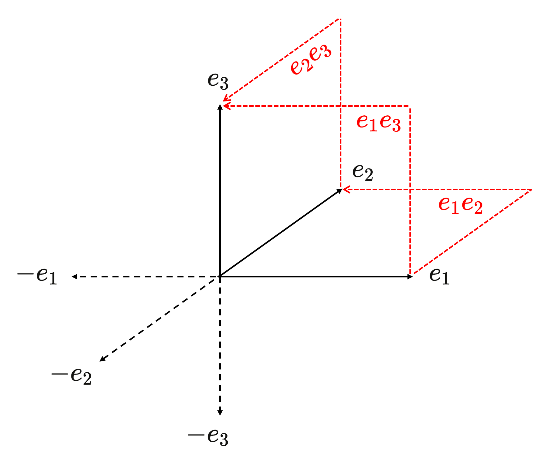
This diagram shows the basic 1-blades (unbroken black arrows) and the basic 2-blades (red, dotted, broken arrows) among the blades in the canonical basis for \, G(e_1, e_2, e_3) .
The negatives of the basic 1-blades are shown as dotted black arrows.
The 2-blades \, \textcolor {red} {e_1 e_2} \textcolor {black} {,} \textcolor {red} {e_2 e_3} \textcolor {black} {,} \textcolor {red} {e_1 e_3} \,
represent the directed area within the corresponding squares.
Hence we have for \, k \neq i \, : \, (e_i e_k)^2 = e_i e_k e_i e_k = - e_k e_i e_i e_k = - e_k e_k = -1
///////
The 3D pseudoscalar E :
E = e_1 e_2 e_3 .
E^{-1} = e_3 e_2 e_1 .
E E^{-1} = e_1 e_2 e_3 e_3 e_2 e_1 = 1 .
E^{-1} E = \, e_3 e_2 e_1 e_1 e_2 e_3 = 1 .
E^2 = e_1 e_2 e_3 e_1 e_2 e_3 = - e_2 e_1 e_3 e_1 e_2 e_3 = e_2 e_3 e_1 e_1 e_2 e_3 = e_2 e_3 e_2 e_3= - e_3 e_2 e_2 e_3 \, = \, - e_3 e_3 = -1 .
(E^{-1})^2 = e_3 e_2 e_1 e_3 e_2 e_1 = - e_3 e _2 e_1 e_3 e_1 e_2 = e_3 e _2 e_1 e_1 e_3 e_2 = e_3 e_2 e_3 e_2= - e_3 e_2 e_2 e_3 \, = \, - e_3 e_3 = -1 .
Duality of basis 1-blades:
= - e_3 e_1 e_1 e_2 = - e_3 e_2 = e_2 e_3 = e_2 \wedge e_3 .
{e_2}^* = - e_2 E^{-1} = - e_2 e_3 e_2 e_1 = e_3 e_2 e_2 e_1 = e_3 e_1 = e_3 \wedge e_1.
\, {e_3}^*= - e_3 E^{-1} = - e_3 e_3 e_2 e_1 = - e_2 e_1 = e_1 e_2 = e_1 \wedge e_2 .
Duality of basis 2-blades:
{e_1}^{**} = ({e_2 e_3})^* = e_2 e_3 E^{-1} = e_2 e_3 e_3 e_2 e_1 = e_2 e_2 e_1 = e_1.
{e_2}^{**} = ({e_3 e_1})^* = e_3 e_1 E^{-1} = e_3 e_1 e_3 e_2 e_1 = - e_1 e_3 e_3 e_2 e_1 = - e_1 e_2 e_1 = e_2 e_1 e_1 = e_2 .
{e_3}^{**} = ({e_1 e_2})^* = e_1 e_2 E^{-1} = e_1 e_2 e_3 e_2 e_1 = - e_1 e_3 e_2 e_2 e_1 = - e_1 e_3 e_1 = e_3 e_1 e_1 = e_3 .
Checking that duality is equal to complementarity to E under the geometric product :
e_1 {e_1}^* = e_1 e_2 e_3 = E .
e_2 {e_2}^* = e_2 e_3 e_1 = - e_2 e_1 e_3 = e_1 e_2 e_3 = E .
e_3 {e_3}^* = e_3 e_1 e_2 = - e_1 e_3 e_2 = e_1 e_2 e_3 = E .
Duality of general 1-vectors :
a = a_1 e_1 + a_2 e_2 + a_3 e_3 .
a^*= (a_1 e_1 + a_2 e_2 + a_3 e_3)^*= a_1 e_2 e_3 + a_2 e_3 e_1 + a_3 e_1 e_2 .
b = b_1 e_1 + b_2 e_2 + b_3 e_3 .
b^*= (b_1 e_1 + b_2 e_2 + b_3 e_3)^*= b_1 e_2 e_3 + b_2 e_3 e_1 + b_3 e_1 e_2 .
Reordering the factors of the basic 2-blades to use the increasing order gives :
a^* = a_1 e_2 e_3 - a_2 e_1 e_3 + a_3 e_1 e_2 .
b^* = b_1 e_2 e_3 - b_2 e_1 e_3 + b_3 e_1 e_2 .
Outer product of 1-vectors a and b :
a{\wedge}b = (a_1 e_1 + a_2 e_2 + a_3 e_3) \wedge (b_1 e_1 + b_2 e_2 + b_3 e_3) = a_1 b_2 e_1 e_2 + a_1 b_3 e_1 e_3 + a_2 b_1 e_2 e_1 + a_2 b_3 e_2 e_3 + a_3 b_1 e_3 e_1 + a_3 b_2 e_3 e_2 = (a_1 b_2 - a_2 b_1) e_1 e_2 + (a_1 b_3 - a_3 b_1) e_1 e_3 + (a_2 b_3 - a_3 b_2) e_2 e_3 . In summary :
a{\wedge}b = (a_1 b_2 - a_2 b_1) e_1 e_2 + (a_1 b_3 - a_3 b_1) e_1 e_3 + (a_2 b_3 - a_3 b_2) e_2 e_3 .
Dualisation of a{\wedge}b :
Since ({e_2 e_3})^* = e_1, ({e_1 e_3})^* = - e_2, and ({e_1 e_2})^* = e_3 we have :
(a{\wedge}b)^* =
= (a_1 b_2 - a_2 b_1) (e_1 e_2)^* + (a_1 b_3 - a_3 b_1) (e_1 e_3)^* + (a_2 b_3 - a_3 b_2) (e_2 e_3)^*
= (a_1 b_2 - a_2 b_1) e_3 - (a_1 b_3 - a_3 b_1) e_2 + (a_2 b_3 - a_3 b_2) e_1 .
Comparison with the cross product of a and b :
a{\times}b = (a_1 b_2 - a_2 b_1) e_3 - (a_1 b_3 - a_3 b_1) e_2 + (a_2 b_3 - a_3 b_2) e_1 .
From this comparison we can conclude that :
(a{\wedge}b)^* = a{\times}b .
(a{\times}b)^* = a{\wedge}b .
///////
QUATERNIONS ARE ISOMORPHIC TO EVEN SUBALGEBRA OF \, G(e_1, e_2, e_3) \, .
Addition rule for the even subalgebra of \, G(e_1, e_2, e_3) \, :
\, (\alpha \textcolor {red} 1 + \alpha_{12} \textcolor {red} {e_1 e_2} + \alpha_{23} \textcolor {red} {e_2 e_3} \, + \alpha_{13} \textcolor {red} {e_1 e_3}) \, +
\, (\alpha' \textcolor {red} 1 +\alpha'_{12} \textcolor {red} {e_1 e_2} + \alpha'_{23} \textcolor {red} {e_2 e_3} + \alpha'_{13} \textcolor {red} {e_1 e_3}) \stackrel {\mathrm{def}}{=} \,
\, (\alpha+\alpha') \textcolor {red} 1 + (\alpha_{12}+\alpha'_{12}) \textcolor {red} {e_1 e_2} + (\alpha_{23}+\alpha'_{23}) \textcolor {red} {e_2 e_3} + (\alpha_{13}+\alpha'_{13}) \textcolor {red} {e_1 e_3} .
Multiplication table for the even subalgebra of \, G(e_1, e_2, e_3) \, :
\, \begin{matrix} * & ~ & \textcolor {red} 1 & \textcolor {red} {e_1 e_2} & \textcolor {red} {e_2 e_3} & \textcolor {red} {e_1 e_3} \\ & & & & & & \\ \textcolor {red} 1 & ~ & \textcolor {red} 1 & \textcolor {red} {e_1 e_2} & \textcolor {red} {e_2 e_3} & \textcolor {red} {e_1 e_3} \\ \textcolor {red} {e_1 e_2} & ~ & \textcolor {red} {e_1 e_2} & - \textcolor {red} 1 & \textcolor {red} {e_1 e_3} & - \textcolor {red} {e_2 e_3} \\ \textcolor {red} {e_2 e_3} & ~ & \textcolor {red} {e_2 e_3} & - \textcolor {red} {e_1 e_3} & - \textcolor {red} 1 & \textcolor {red} {e_1 e_2} \\ \textcolor {red} {e_1 e_3} & ~ & \textcolor {red} {e_1 e_3} & \textcolor {red} {e_2 e_3} & - \textcolor {red} {e_1 e_2} & - \textcolor {red} 1 \, \end{matrix} \, .
Multiplication table for the quaternions:
\, \begin{matrix} * & ~ & \bold 1 & \;\; \bold i & \;\; \bold j & \, \;\, \bold k \\ & & & & & & \\ \bold 1 & ~ & \bold 1 & \;\; \bold i & \;\; \bold j & \;\; \bold k \\ \bold i & ~ & \bold i & - \bold 1 & \;\; \bold k & - \bold j \\ \bold j & ~ & \bold j & - \bold k & - \bold 1 & \;\; \bold i \\ \bold k & ~ & \bold k & \;\; \bold j & - \bold i & - \bold 1 \, \end{matrix} \, .
Substituting \, \bold 1 = \textcolor {red} {1} \, , \, \bold i = \textcolor {red} {e_1 e_2} \, , \, \bold j = \textcolor {red} {e_2 e_3} \, , \bold k = \textcolor {red} {e_1 e_3} \, we see that the addition rule above for the even subalgebra of \, G(e_1, e_2, e_3) \, becomes the addition rule for quaternions. Moreover, comparing the two multiplication tables, we see that they are isomorphic. Therefore the quaternions and the even subalgebra of \, G(e_1, e_2, e_3) \, are isomorphic as algebras, and therefore they represent the same mathematical structure.
///////
7.2 ROTATIONS OF SUBSPACES
(based on GA for Computer Science, p.169)
Having reflections as a sandwiching product leads naturally to the representation of rotations. For by a well-known theorem, any rotation can be represented as the product of an even number of reflections. In geometric algebra, this statement can be converted immediately into a computational form.
Rotors as double reflections
Two reflections make a rotation, even in {\mathbb{R}}^3 (see figure 7.2). Since the product of an even number of reflections absorbs any sign, we may make these reflections either both line reflections \mathbf{a} \, x \, {\mathbf{a}}^{-1} or both (dual) hyperplane reflections - \mathbf{a} \, x \, {\mathbf{a}}^{-1} , whichever feels most natural or is easiest to visualize. The figure uses line reflections.
///////
7.2.2 ROTORS PERFORM ROTATIONS (p.172)
It is natural to relate the rotor \mathbf{b}/\mathbf{a} to the geometrical relationship between two vectors: their common plane \mathbf{b} \wedge \mathbf{a} and their relative angle. We can use those geometric elements to encode it algebraically, by deveoping the geometric product of the unit vectors, we have \mathbf{b}/\mathbf{a} = \mathbf{b} \mathbf{a} , and compute
R = \mathbf{b} \, \mathbf{a} = \mathbf{b} \cdot \mathbf{a} + \mathbf{b} \wedge\mathbf{a} = \cos(ø/2) - \mathbf{I} \sin(ø/2), \;\;\;\;\;\;\;\; \;\;\;\; (7.4)
where ø/2 is the angle from \mathbf{a} to \mathbf{b} and \mathbf{I} is the unit 2-blade for the (\mathbf{a} \wedge \mathbf{b})-plane. This rotor involving the angle ø/2 actually rotates over ø (as Figure 7.2 suggests, and as we will show below.
The action of a rotor may appear a bit magical at first. It is good to see in detail how the sandwiching works to produce a rotation of a vector \mathbf{x} in a Euclidean space.
To do so, we introduce notations for the various components of \mathbf{x} relative to the rotation plane. What we would hope when we apply the rotor to \mathbf{x} is that
• The component of \mathbf{x} perpendicular to the rotation plane,
the rejection {\mathbf{x}}_{\uparrow} defined by {\mathbf{x}}_{\uparrow} \equiv (\mathbf{x} \wedge \mathbf{I}) / \mathbf{I} , remains unchanged.
• The component of \mathbf{x} within the rotation plane,
the projection {\mathbf{x}}_{\parallel} \equiv ( \mathbf{x} \, \lrcorner \, \mathbf{I} ) / \mathbf{I} , gets shortened by a scaling factor of \cos(ø) .
• A component of \mathbf{x} perpendicular to the projection in the rotation plane,
{\mathbf{x}}_{\perp} \equiv \mathbf{x} \, \lrcorner \, \mathbf{I} = {\mathbf{x}}_{\parallel} \mathbf{I} , gets added with a scaling factor of \sin(ø) .
It seems a lot to ask of the simple formula R \mathbf{x} \tilde{R} , but we can derive that this is indeed precisely what it does. The structure of the derivations is simplified when we define c \equiv \cos(ø/2) , s \equiv \sin(ø/2) , and note beforehand that both the rejection and projection operators satisfy the commutation relations {\mathbf{x}}_{\uparrow} \mathbf{I} = \mathbf{I} {\mathbf{x}}_{\uparrow} and {\mathbf{x}}_{\parallel} \mathbf{I} = - \mathbf{I} {\mathbf{x}}_{\parallel} (these relations actually define them fully, by the relationships of Section 6.3.1). Also, we have seen in (6.4) that in a Euclidean space {\mathbf{I}}^2 = -1 , which is essential to make the whole thing work. Then
\begin{aligned} R \mathbf{x} \tilde{R} &= R ( {\mathbf{x}}_{\uparrow} + {\mathbf{x}}_{\parallel} ) \tilde{R} \\ &= (c - s \, \mathbf{I}) ( {\mathbf{x}}_{\uparrow} + {\mathbf{x}}_{\parallel} ) (c + s \, \mathbf{I}) \\ &= c^2 {\mathbf{x}}_{\uparrow} - s^2 ( \mathbf{I} \, {\mathbf{x}}_{\uparrow} \, \mathbf{I} ) + c s ( {\mathbf{x}}_{\uparrow} \, \mathbf{I} - \mathbf{I} \, {\mathbf{x}}_{\uparrow} ) + c s ( {\mathbf{x}}_{\parallel} \, \mathbf{I} - \mathbf{I} \, {\mathbf{x}}_{\parallel} ) + c^2 \, {\mathbf{x}}_{\parallel} \ -s^2 ( \mathbf{I} \, {\mathbf{x}}_{\parallel} \, \mathbf{I} ) \\ &= (c^2 + s^2) {\mathbf{x}}_{\uparrow} + (c^2 - s^2) {\mathbf{x}}_{\parallel} + 2c s \, {\mathbf{x}}_{\parallel} \, \mathbf{I}) \\ &= {\mathbf{x}}_{\uparrow} + \cos(ø ) \, {\mathbf{x}}_{\parallel} + \sin(ø) \, {\mathbf{x}}_{\perp} \end{aligned} \,
which is the desired result. Note especially how the 1-vector {\mathbf{x}}_{\perp} , which was not originally present, is generated automatically. It is very satisfying that the whole process is driven by the algebraic commutation rules that encode the various geometrical perpendicularity and containment relationship. This shows that we truly have an algebra capable of mimicking geometry.
7.3.5 UNIT QUATERNIONS SUBSUMED (p.181)
////////
Explicit correspondence between rotors and quaternions
(based on GA for Computer Science)
Let us spell out the correspondence between rotors and quaternions precisely. A quaternion consists of two parts, a scalar part and a complex vector part:
quaternion: q = q_0 + \mathbf{\overrightarrow{q}} .
We will consider only unit quaternions, characterized by {q_0}^2 + { || \mathbf{\overrightarrow{q}} || }^2 = 1 . The nonscalar part of a unit quaternion is often seen as a kind of vector that denotes a rotation axis, but expressed in a strange basis of complex vector quantities i, j, k, that square to -1 and anticommute. For us, \mathbf{\overrightarrow{q}} and its basis elements are not vectors but basis 2-blades of the coordinate planes:
i = - {\mathbf{E}}_3 \, e_1 = e_3 e_2, \; j = - {\mathbf{E}}_3 \, e_2 = e_1 e_3, \; k= - {\mathbf{E}}_3 \, e_3 = e_2 e_1 .
Note that i j = k and cyclic, and i j k = 1 . The three components of an element on this 2-blade basis represent not the rotation unit axis vector \mathbf{e} , but the rotation plane \mathbf{I} . The two are related simply by geometric duality (i.e., by quantitative orthogonal complement) as
axis \mathbf{e} to 2-blade \mathbf{I}: \;\; \mathbf{e} \equiv {\mathbf{I}}^* = \mathbf{I} \, {{\mathbf{E}}_3}^{-1} , so \mathbf{e} \, {\mathbf{E}}_3 = \mathbf{I} ,
and their coefficients are similar, though on totally different bases (basis vectors for the axis and basis 2-blades for the rotation plane \mathbf{I} ).
The standard notation for a unit quaternion: q = q_0 + \mathbf{\overrightarrow{q}} separates into a scalar part q_0 and a supposedly complex vector part \mathbf{\overrightarrow{q}} denoting the axis. In geometric algebra this naturally corresponds to a rotor R = q_0 - \mathbf{q} {\mathbf{E}}_3 , having a scalar part and a 2-blade part:
\;\;\;\;\;\; unit quaternion: q = q_0 + \mathbf{\overrightarrow{q}} \;\;\; \leftrightarrow \;\;\;\ rotor: \; q_0 - \mathbf{q} {\mathbf{E}}_3 .
(The minus sign derives from the rotor definition (7.4). In the latter, \mathbf{q} is now a real vector denoting the rotation axis. When combining these quantities, the common geometric product naturally takes over the role of the rather ad hoc quaternion product. We embed unit quaternions as rotors, perform the multiplication and transfer back:
\begin{aligned} q \, p \, &= \,(q_0 + \mathbf{\overrightarrow{q}}) (p_0 + \mathbf{\overrightarrow{p}}) &\text{(quaternion product)} \\ &\leftrightarrow ( q_0 - \mathbf{q} \, {\mathbf{E}}_3) (p_0 - \mathbf{p} \, {\mathbf{E}}_3 ) &\text{(geometric product)} \\ &= q_0 p_0 + {\left< {\mathbf{E}}_3 \, \mathbf{q} \, {\mathbf{E}}_3 \, \mathbf{p} \right>}_0 - ( \mathbf{q} p_0 + q_0 \mathbf{p} - {\left< {\mathbf{E}}_3 \, \mathbf{q} \, {\mathbf{E}}_3 \, \mathbf{p} \right>}_2 \, {{\mathbf{E}}_3}^{-1} ) {\mathbf{E}}_3 & \\ &= q_0 p_0 - {\left<\mathbf{q} \, \mathbf{p} \right>}_0 - ( \mathbf{q} p_0 + q_0 \mathbf{p} + {\left<\mathbf{q} \, \mathbf{p} \right>}_2 \, {{\mathbf{E}}_3}^{-1} ) {\mathbf{E}}_3 & \\ &= q_0 p_0 - \mathbf{q} \cdot \mathbf{p} - ( \mathbf{q} p_0 + q_0 \mathbf{p} + \mathbf{q} \times \mathbf{p}) {\mathbf{E}}_3 & \\ &\leftrightarrow ( q_0 p_0 - \mathbf{\overrightarrow{q}} \cdot \mathbf{\overrightarrow{p}} ) + ( p_0 \mathbf{\overrightarrow{q}} + q_0 \mathbf{\overrightarrow{p}} + \mathbf{\overrightarrow{q}} \times \mathbf{\overrightarrow{p}} ) & \end{aligned} (7.11)
There is one conversion step of the above steps that may require some extra explanation: {\left<\mathbf{q} \mathbf{p} \right>}_2 E^{-1} = \mathbf{q} \times \mathbf{p} , by (3.28). The inner product and cross product in (7.11) are just defined as the usual combinations of the complex vectors.
With the above, we have retrieved the usual multiplication formula from the quaternion literature, but using only quantities from the real geometric algebra of the 3-D Euclidean space {\mathbb{R}}^{(3,0)} . This shows that the unit quaternion product is really just the geometric product on rotors. The quaternion product formula betrays its three-dimensional origin clearly in its use of the cross product, whereas the geometric product is universal and works for rotors in n-dimensional space.
The geometric algebra method gives us a more natural context to use the quaternions. In fact, we don’t use them, for like complex numbers in 2-D they are only half of what is needed to do Euclidean geometry in 3-D. We really need both rotation operators and vectors, separately, in a clear algebraic relationship. The rotation operators are rotors that obey the same multiplication rule as unit quaternions; the structural similarity between (7.9) and (7.11) should be obvious. This is explored in structural exercise 10. Of course, the rule must be the same, since both rotors and quaternions can effectively encode the composition of 3-D rotations.
We summarize the advantages of rotors: In contrast to quaternions, rotors can rotate k-dimensional subspaces. Geometrically, they provide us with a clear and real visualization of unit quaternions, exposed in the previous section as half-angle arcs on a rotational sphere that is visible in 3-D space as opposed to being hidden in 4-D space. These rotations can be composed by sliding and and addition, using classical spherical geometry (see [29] Appendix A).
It is a pity that the mere occurrence of of some elements that square to -1 appears to have stifled all sensible attempts of visualization in the usual approach to quaternions, making them appear unnecessarily complex. Keep using them if you already did, but at least do so with a real understanding of what they are.
//////// Safety copy
\begin{aligned} q \, p \, &= \,(q_0 + \mathbf{\overrightarrow{q}}) (p_0 + \mathbf{\overrightarrow{p}}) &\text{(quaternion product)} \\ &\leftrightarrow ( q_0 - \mathbf{q} \, {\mathbf{E}}_3) (p_0 - \mathbf{p} \, {\mathbf{E}}_3 ) &\text{(geometric product)} \\ &= q_0 p_0 + {\left< {\mathbf{E}}_3 \, \mathbf{q} \, {\mathbf{E}}_3 \, \mathbf{p} \right>}_0 - ( \mathbf{q} p_0 + q_0 \mathbf{p} - {\left< {\mathbf{E}}_3 \, \mathbf{q} \, {\mathbf{E}}_3 \, \mathbf{p} \right>}_2 \, {{\mathbf{E}}_3}^{-1} ) {\mathbf{E}}_3 & \\ &= q_0 p_0 - {\left<\mathbf{q} \, \mathbf{p} \right>}_0 - ( \mathbf{q} p_0 + q_0 \mathbf{p} + {\left<\mathbf{q} \, \mathbf{p} \, \right>}_2 \, {{\mathbf{E}}_3}^{-1} ) {\mathbf{E}}_3 & \\ &= q_0 p_0 - \mathbf{q} \cdot \mathbf{p} - ( \mathbf{q} p_0 + q_0 \mathbf{p} + \mathbf{q} \times \mathbf{p}) {\mathbf{E}}_3 & \\ &\leftrightarrow ( q_0 p_0 - \mathbf{\overrightarrow{q}} \cdot \mathbf{\overrightarrow{p}} ) + ( p_0 \mathbf{\overrightarrow{q}} + q_0 \mathbf{\overrightarrow{p}} + \mathbf{\overrightarrow{q}} \times \mathbf{\overrightarrow{p}} ) & \end{aligned} (7.11)
///////
7.4 EXPONENTIAL REPRESENTATION OF ROTORS (p. 182)
In Section 7.3.1, we made a basic rotor as the ratio between two unit vectors, which is effectively their geometric product. Multiple applications then lead to:
In a Euclidean space {\mathbb{R}}^{n,0} , a rotor is the geometric product of an even number of unit vectors.
The inverse of a rotor composed of such unit vectors is simply its reverse. This is not guaranteed in a general metrics, which has unit vectors that square to -1 . But if R \, \tilde{R} would be -1 , R would not even produce a linear transformation, for it would reverse the sign of scalars. Therefore, we should prevent this and have as a definition for the more general spaces:
A rotor R is a geometric product of an even number of unit vectors, such that R \, \tilde{R} = 1 .
Even within those more sharply defined rotors, mathematicians such as Riesz [52] make a further important distinction between rotors that are “continuously connected to the identity” and those that are not. This property implies that ssome rotors can be performed gradually in small amounts (such as rotations), but that in the more general metrics there are also rotors that are like reflections and generate discontinous motion. Only the former rotors are candidates for the proper orthogonal transformations that we hope to represent by rotors.
You can always attempt to construct rotors as products of unit vectors, but checking whether you have actually created a proper rotor becomes cumbersome. Fortunately, there is an alternative representation in which this is trivial, and moreover, it often corresponds more directly to the givens in a geometric problem. It is the exponential representation, which computes a Euclidean rotor immediately from its intended rotation plane and angle. That construction generalizes unchanged to other metrics.
7.4.1 PURE ROTORS AS EXPONENTIALS OF 2-BLADES (p. 183)
We have seen how in Euclidean 3-D space, a rotor R_{\mathbf{I} ø } can be written as the sum of a scalar and a 2-blade, involving a cosine and a sine of the scalar angle ø . We can also express the rotor in terms of its bivector angle using the exponential form of the rotor:
\;\;\;\;\;\;\;\;\; R_{\mathbf{I} ø } = \cos(ø/2) - \mathbf{I} \, \sin(ø/2) = e^{-\mathbf{I} ø/2}. \;\;\;\;\;\;\;\;\;\;\;\;\;\;\; (7.12)
The exponential on the right-hand side is defined by the usual power series. The correctness of this exponential rewriting can be demonstrated by collecting the terms in this series with and without a net factor of \mathbf{I} . Because {\mathbf{I}}^2 = -1 in the Euclidean metric, that leaves the familiar scalar power series of sine and cosine. To show the structure of this derivation more clearly, we define \psi = ø/2 .
\begin{aligned} e^{\mathbf{I} \psi} &= 1 + \dfrac{ \mathbf{I} \psi} {1!} + \dfrac { { { ( \mathbf{I} \psi} ) }^2 } {2!} + \dfrac { { { ( \mathbf{I} \psi} ) }^3 } {3!} + \cdots, \\ &= ( 1 - \dfrac { \psi^2 } {2!} + \dfrac { \psi^4 } {4!} - \cdots) + \mathbf{I} \, (\dfrac{\psi} {1!} - \dfrac { \psi^3 } {3!} + \dfrac { \psi^5 } {5!} - \cdots ) \\ &= \cos(\psi) + \mathbf{I} \, \sin(\psi). \end{aligned} \;\;\;\;\;\;\;\;\;\;\;\; (7.13)
After some practice, you will no longer need to use the scalar plus bivector form of the rotor R_{\mathbf{I} ø } to perform derivations but will be able to use its exponential form instead. For instance, if you have the components {\mathbf{x}}_{\parallel} of a vector \mathbf{x} that is contained in \mathbf{I} , then {\mathbf{x}}_{\parallel} \, \mathbf{I} = - \mathbf{I} \, {\mathbf{x}}_{\parallel} .
From this you should dare to state the commutation rule for the versor R_{\mathbf{I} ø } immediately as {\mathbf{x}}_{\parallel} R_{\mathbf{I} ø } = R_{-\mathbf{I} ø } \, {\mathbf{x}}_{\parallel} and use it to show directly that
\;\;\;\;\;\;\;\;\; R_{\mathbf{I} ø } \, {\mathbf{x}}_{\parallel} \, \widetilde{R_{\mathbf{I} ø } } = e^{- \mathbf{I} ø/2} \, {\mathbf{x}}_{\parallel} \, e^{\mathbf{I} ø/2} = {\mathbf{x}}_{\parallel} \, e^{\mathbf{I} ø/2} \, e^{\mathbf{I} ø/2} = {\mathbf{x}}_{\parallel} \, e^{\mathbf{I} ø} ,
or, if you would rather, e^{- \mathbf{I} ø} \, {\mathbf{x}}_{\parallel} . So within the \mathbf{I}-plane, the formula \mathbf{x} \mapsto \mathbf{x} \, e^{\mathbf{I} ø} performs a rotation. This result is (7.6), now with a more compact computational dervation.
Clearly, the exponential representation in (7.13) is algebraically isomorphic to the exponential representation of a unit complex numer by the correspondence exposed in Section 7.3.2. The result
\;\;\;\;\;\;\;\;\; e^{ i \pi } + 1 = 0 ,
famously involving “all” relevant computational elements of elementary calculus, is obtained from (7.12) by setting i = -\mathbf{I} and ø = 2 \pi , as e^{ - \mathbf{I} \pi } = -1 . Its geometric meaning is that a rotation over ø = 2 \pi in any plane \mathbf{I} has the rotor -1 not +1 ; remember Dirac’s belt trick !).
7.4.2 TRIGONOMETRIC AND HYPERBOLIC FUNCTIONS (p.184)
//////
7.4.3 ROTORS AS EXPONENTIALS OF BIVECTORS (p.185)
//////
7.5.1 REFLECTION BY SUBSPACES (p.188)
//////
7.5.2 SUBSPACE PROJECTION AS SANDWICHING (p.190)
//////
7.6 VERSORS GENERATE ORTHOGONAL TRANSFORMATIONS (p.191)
//////
7.6.1 THE VERSOR PRODUCT (p.192)
//////
7.6.2 EVEN AND ODD VERSORS (p.193)
//////
7.6.3 ORTHOGONAL TRANSFORMATIONS ARE VERSOR PRODUCTS (p.193)
//////
7.6.4 VERSORS, BLADES, ROTORS, AND SPINORS (p.195)
//////
7.7 THE PRODUCT STRUCTURE OF GEOMETRIC ALGEBRA (p.196)
7.7.1 THE PRODUCTS SUMMARIZED (p.196)
//////
7.7.2 GEOMETRIC ALGEBRA VERSUS CLIFFORD ALGEBRA (p.198)
//////
7.7.3 BUT IS IT EFFICIENT? (p.199)
//////