This is a sub-page of our page on Algebra.
///////
Sub-pages of this page
• Matrices and Gaussian Elimination
///////
Related KMR pages:
Geometry:
• Linear Transformations
• Projective Geometry
• Line Geometry
Combinatorics:
• Combinatorial Clifford Algebra
• Foresight and Hindsight Process Manager
///////
Other related sources of information:
• Linear Algebra and its Applications, Gilbert Strang (1986), Third Edition (1988).
• Matrix Algebra
• Adjacency Matrices
• HMC Mathematics Online Tutorial on Matrix Algebra (Harvey Mudd College)
• The Matrix Calculus You Need For Deep Learning (by Terence Parr and Jeremy Howard)
///////
The Applications of Matrices | What I wish my teachers told me way earlier
(Zach Star on YouTube):
///////
/////// Quoting Strang (1986, p.63):
2.1 VECTOR SPACES AND SUBSPACES
Elimination can simplify, one entry at a time, the linear system \, A x = b . Fortunately it also simplifies the theory. The basic questions of existence and uniqueness – Is there one solution, or no solution, or an infinity of solutions? – are much easier to answer after elimination. We need to devote one more section to those questions; then that circle of ideas will be complete. But the mechanics of elimination produces only one kind of understanding of a linear system, and our chief object is to achieve a different and deeper understanding. This chapter may be more difficult than the first one. It goes to the heart of linear algebra.
First we need the concept of a vector space. To introduce that idea we start immediately with the most important vector spaces. They are denoted by \, \mathbf { R^1, R^2, R^3,} \, ... \, ; there is one for every positive integer. The space \, \mathbf R^n \, consists of all column vectors with \, n \, components. (The components are real numbers.) The space \, \mathbf R^2 \, is represented by the usual \, xy \, plane; the two components of the vector become the \, x \, and \, y \, coordinates of the corresponding point. \, \mathbf R^3 \, is equally familiar, with the three components giving a point in three-dimensional space. The one-dimensional space \, \mathbf R^1 \, is a line.
The valuable thing for linear algebra is that the extension to \, n \, dimensions is so straightforward; for a vector in seven-dimensional space \, \mathbf R^7 \, we just need to know the seven components, even if the geometry is hard to visualize.
Within these spaces, and within all vector spaces, two operations are possible:
We can add any two vectors and we can multiply vectors by scalars.
For the spaces \, \mathbf R^n \, these operations are done a component at a time. If \, x \, is the vector in \, \mathbf R^4 \, with components \, 1, 0, 0, 3 , then \, 2 x \, is the vector with the components \, 2, 0, 0, 6 . A whole series of properties could be verified – the commutative law \, x + y = y + x , or the existence of a “zero vector” satisfying \, 0 + x = x , or the existence of a vector “ -x ” satisfying \, -x + x = 0 . Of all these properties, eight (including those three) are fundamental; the full list is given in Exercise 2.1.5.
Formally, a real vector space is a set of “vectors” together with rules for vector addition and multiplication by real numbers. The addition and multiplication must produce vectors that are within the space, and they must satisfy the eight conditions.
Normally our vectors belong to one of the spaces \, \mathbf R^n ; they are ordinary column vectors. The formal definition, however, allows us to think of other things as vectors – provided that addition and scalar multiplication are all right. We give three examples:
(i) The infinite-dimensional space \, \mathbf R^{\infty} . Its vectors have infinitely many components as in \, x = (1, 2, 1, 2, 1, ...) , but the laws of addition and multiplication stay unchanged.
(ii) The space of 3 by 2 matrices. In this case the “vectors” are matrices! We can add two matrices and \, A + B = B + A , and there is a zero matrix, and so on. This space is almost the same as \, \mathbf R^6 . (The six components are arranged in a rectangle instead of a column.) Any choice of \, m \, and \, n \, would give, as a similar example, the vector space of all \, m \, by \, n \, matrices.
(iii) The space of functions \, f(x) . Here we admit all functions \, f \, that are defined on a fixed intervals, say \, 0 \le x \le 1 . The space includes \, f(x) = x^2, g(x) = \sin x , their sum \, (f + g)(x) = x^2 + \sin x , and all multiples like \, 3 x^2 \, and \, - \sin x . The vectors are functions, and again the dimension is infinite – in fact it is a larger infinity than for \, \mathbf R^{\infty} .
/////// End of quote from Strang (1986)
/////// Quoting Strang (1986, p. 65):
We now come to the key examples of subspaces. They are tied directly to a matrix \, A \, and they give information about the system \, Ax = b . In some cases they contain vectors with \, m \, components, like the columns of \, A ; then they are subspaces of \, \mathbf R^m . In other cases the vectors have \, n \, components, like the rows of \, A \, (or like \, x \, itself); those are subspaces of \, \mathbf R^n . We illustrate by a system of three equations in two unknowns:
\, \begin{bmatrix} 1 & 0 \\ 5 & 4 \\ 2 & 4 \end{bmatrix} \begin{bmatrix} u \\ v \end{bmatrix} = \begin{bmatrix} b_1 \\ b_2 \\ b_3 \end{bmatrix} .
If there were more unknowns than equations, we might expect to find plenty of solutions (although that is not always so). In the present case there are more equations than unknowns – and we must expect that usually there will be no solution. A system with \, m > n \, will be solvable only for certain right-hand sides, in fact, for a very “thin” subset of all possible three-dimensional vectors \, b . We want to find that subset of \, b ‘s.
One way of describing this subset is so simple that it is easy to overlook.
2A The system \, Ax = b \, is solvable if and only if the vector \, b \, can be expressed as a combination of the columns of \, A .
This description involves nothing more than a restatement of the system \, Ax = b , writing it in the following way:
\, u \begin{bmatrix} 1 \\ 5 \\ 2 \end{bmatrix} + v \begin{bmatrix} 0 \\ 4 \\ 4 \end{bmatrix} = \begin{bmatrix} b_1 \\ b_2 \\ b_3 \end{bmatrix} .
These are the same three equations in two unknowns. But now the problem is seen to be this: Find numbers \, u \, and \, v \, that multiply the first and the second columns of \, A \, to produce the vector \, b . The system is solvable exactly when such coefficients exist, and the vector \, (u, v) \, is the solution \, x .
Thus the subset of attainable right-hand sides \, b \, is the set of all combinations of the columns of \, A . One possible right side is the first column itself; the weights are \, u = 1 \, and \, v = 0 . Another possibility is the second column: \, u = 0 \, and \, v = 1 . A third is the right side \, b = 0 ; the weights are \, u = 0 , \, v = 0 \, (and with that trivial choice, the vector \, b = 0 \, will be attainable no matter what the matrix is).
Now we have to consider all combinations of the two columns and we describe the result geometrically: \, Ax = b \, can be solved if and only if \, b \, lies in the plane that is spanned by the two column vectors of \, A (Fig. 2.1). This is the thin set of attainable \, b . If \, b \, lies off the plane, then it is not a combination of the two columns. In that case \, Ax = b \, has no solution.
What is important is that this plane is not just a subset of \, \mathbf R^3 ; it is a subspace. It is called the column space of \, A . The column space of a matrix consists of all combinations of the columns. It is denoted by \, \mathscr{R}(A) . The equation \, Ax = b \, can be solved if and only if b lies in the column space of \, A . For an \, m by \, n matrix this will be a subspace of \, \mathbf R^m , since the columns have \, m \, components, and the requirements (i) and (ii) for a subspace are easy to check:
(i): Suppose \, b \, and \, b' \, lie in the column space, so that \, Ax = b \, for some \, x \, and \, Ax' = b' \, for some \, x' \, ; \, x \, and \, x' \, just give the combinations which produce \, b \, and \, b' . Then \, A(x + x') = b + b' , so that \, b + b' \, is also a combination of the columns. If \, b \, is column 1 minus column 2, and \, b' \, is twice column 2, then \, b + b' \, is column 1 plus column 2. The attainable vectors are closed under addition, and the first requirement for a subspace is met.
(ii): If \, b \, is in the column space, so is any multiple \, cb . If some combination of columns produces \, b \, (say \, Ax = b ), then multiplying every coefficient in the combination by \, c \, will produce \, cb \, . In other words, \, A(cb) = cb .
Geometrically, the general case is like Fig. 2.1 – except that the dimensions may be very different. We need not have a two-dimensional plane within three-dimensional space. Similarly, the perpendicular to the column space, which we drew in Fig 2.1, may not always be a line. At one extreme, the smallest possible column space comes from the zero matrix \, A = 0 . The only vector in its column space (the only combination of the columns) is \, b = 0 , and no other choice of \, b \, allows us to solve \, 0 x = b .
At the other extreme, suppose \, A \, is the 5 by 5 identity matrix. Then the column space is the whole of \, \mathbf R^5 ; the five columns of the identity matrix can combine to produce any five-dimensional vector \, b . This is not at all special to the identity matrix:
Any 5 by 5 matrix which is nonsingular will have the whole of \, \mathbf R^5 \, as its column space.
For such a matrix we can solve \, Ax = b \, by Gaussian elimination; there are five pivots. Therefore every \, b \, is in the column space of a nonsingular matrix.
You can see how Chapter 1 is contained in this chapter. There we studied the most straightforward (and most common) case, an \, n \, by \, n \, matrix whose column space is \, \mathbf R^n . Now we allow also singular matrices, and rectangular matrices of any shape: the column space is somewhere between zero space and the whole space. Together with its perpendicular space, it gives one of our two approaches to understanding \, Ax = b .
The Nullspace of \, A
The second approach to \, Ax = b \, is “dual” to the first. We are concerned not only with which right sides \, b \, are attainable, but also with the set of solutions \, x \, that attain them. The right side \, b = 0 \, always allows the particular solution \, x = 0 , but there may be infinitely many other solutions. (There always are, if there are more unknowns than equations \, n > m .)
The set of solutions to \, Ax = 0 \, is itself a vector space – the nullspace of \, A .
The nullspace of a matrix \, A \, consists of all vectors \, x \, such that \, A x = 0 . It is denoted by \, \mathscr{N}(A) . It is a subspace of \, \mathbf R^n , just as the column space was a subspace of \, \mathbf R^5 .
/////// End of quote from Strang (1986)
/////// Quoting Strang (1986, p. 90):
The previous section dealt with definitions rather than constructions. We know what a basis is, but not how to find one. Now, starting from an explicit description of a subspace, we would like to compute an explicit basis.
Subspaces are generally described in one of two ways. First, we may be given a set of vectors that span the [sub]space; this is the case for the column space, when the columns are specified. Second, we may be given a list of constraints on the subspace; we are told, not which vectors are in the [sub]space, but which conditions they must satisfy. The nullspace consists of all vectors that satisfy \, Ax = 0 , and each equation in this system represents a constraint. In the first description, there may be useless columns; in the second description there may be repeated constraints. In neither case is it possible to write down a basis by inspection, and a systematic procedure is necessary.
The reader can guess what that procedure will be. We shall show how to find, from the \, L \, and \, U \, (and \, P \, ) which are produced by elimination, a basis for each of the subspaces associated with \, A . Then, even if it makes this section fuller than the others, we have to look at the extreme case:
When the rank is as large as possible, \, r = n \, or \, r = m \, or \, r = m = n ,
the matrix has a left-inverse \, B \, or a right inverse \, C \, or a two-sided inverse \, A^{-1} .
To organize the whole discussion, we consider each of the four fundamental subspaces in turn. Two of them are familiar and two are new.
1. The column space of \, A , denoted by \, \mathscr{R}(A) .
2. The nullspace of \, A , denoted by \, \mathscr{N}(A) .
3. The row space of \, A , which is the column space of \, A^\text{T} .
It is \, \mathscr{R}(A^\text{T}) , and it is spanned by the rows of \, A .
4. The left nullspace of \, A , which is the nullspace of \, A^\text{T} .
It contains all vectors \, y \, such that \, A^\text{T} y = 0 , and it is written \, \mathscr{N}(A^\text{T}) .
The point about the last two subspaces is that they come from \, A^\text{T} . If \, A \, is an \, m \, by \, n \, matrix, you can see which “host” spaces contain the four subspaces by looking at the number of components:
The nullspace \, \mathscr{N}(A) \, and rowspace \, \mathscr{R}(A^\text{T}) \, are subspaces of \, \mathbf {R^n} .
The left nullspace \, \mathscr{N}(A^\text{T}) \, and column space \, \mathscr{R}(A) \, are subspaces of \, \mathbf {R^m} .
The rows have \, n \, components and the columns have \, m .
/////// End of quote from Strang (1986)
/////// Quoting Strang (1986, p. 95):
Fundamental Theorem of Linear Algebra, Part I
1. \, \mathscr{R}(A) \, = column space of \, A ; dimension \, r
2. \, \mathscr{N}(A) \, = nullspace of \, A ; dimension \, n - r
3. \, \mathscr{R}(A^\text{T}) \, = row space of \, A ; dimension \, r
4. \, \mathscr{N}(A^\text{T}) \, = left nullspace of \, A ; dimension \, m - r
/////// End of quote from Strang (1986)
/////// Quoting Strang (1986, p. 138):
DEFINITION Given a subspace \, V \, of \, \mathbf R^n , the space of all vectors orthogonal to \, V \,
is called the orthogonal complement of \, V \, and denoted by \, V^{\bot} .
Using this terminology, the nullspace is the orthogonal complement of the row space: \, \mathscr{N}(A) = (\mathscr{R}(A^\text{T}))^{\bot} \, . At the same time, the opposite relation also holds: The row space contains all vectors that are orthogonal to the nullspace.
This is not so obvious, since solving \, A x = 0 \, we started with the row space and found all \, x \, that were orthogonal to it; now we are going in the opposite direction. Suppose, however, that some vector \, z \, is orthogonal to the nullspace but is outside the row space. Then adding \, z \, as an extra row of \, A \, would enlarge the row space without changing the nullspace. But we know that there is a fixed formula \, r + (n - r) = n \, :
dim(row space) + dim(nullspace) = number of columns.
Since the last two numbers are unchanged when the new row \, z \, is added, it is impossible for the first one to change either. We conclude that every vector orthogonal to the nullspace is already in the row space: \, \mathscr{R}(A^\text{T}) = (\mathscr{N}(A))^{\bot} \, .
The same reasoning applied to \, A^\text{T} \, produces the dual result: The left nullspace \, \mathscr{N}(A^\text{T}) \, and the column space \, \mathscr{R}(A) \, are orthogonal complements. Their dimensions add upp to \, r + (m - r) = m \, .
This completes the second half of the fundamental theorem of linear algebra. The first half gave the dimensions of the four subspaces, including the fact that row rank = column rank. Now we know that those subspaces are perpendicular, and more than that, they are orthogonal complements.
3D Fundamental Theorem of Linear Algebra Part 2
The nullspace is the orthogonal complement of the row space in \, \mathbf R^n .
The left nullspace is the orthogonal complement of the column space in \, \mathbf R^m .
To repeat, those statements are reversible. The row space contains everything orthogonal to the nullspace. The column space contains everything orthogonal to the left nullspace.
That is just a sentence hidden in the middle of the book, but it decides exactly which equations can be solved! Looked at directly, \, A x = b \, requires \, b \, to be in the column space. Looked at indirectly, it requires \, b \, to be perpendicular to the left nullspace.
/////// End of quote from Strang (1986)
• Matrix transpose isn’t just swapping rows and columns (Mathemaniac on YouTube)
The adjoint \, F^* \, of \, F \, and its representation as the transposed matrix \, A^\text{T} \, :
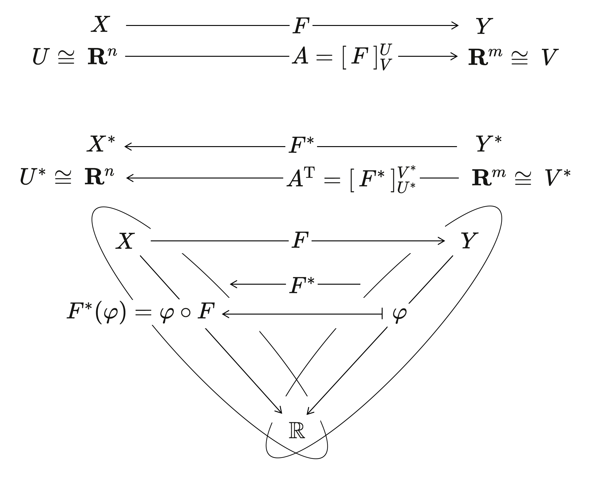
///////
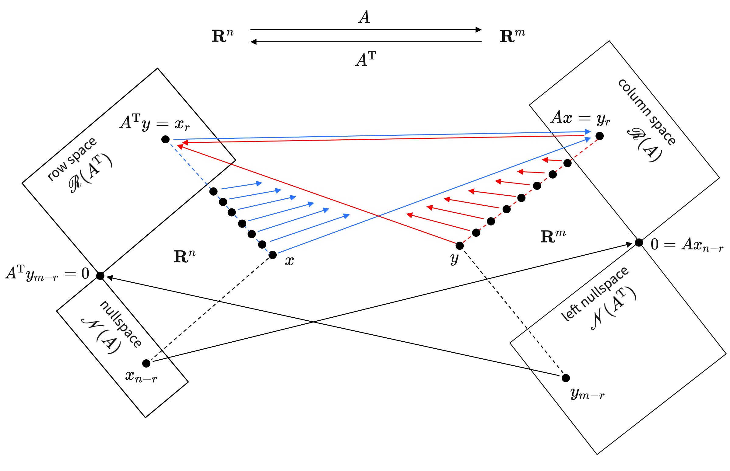
/////// This diagram is based on (Strang, 1986, Fig. 3.4, p. 140):
/////// Connect with Homological Algebra and Category Theory
/////// Quoting Strang, (1986, p.140)
Figure 3.4 summarizes the fundamental theorem of linear algebra. It illustrates the true effect of a matrix – what is happening below the surface of the multiplication \, A x . One part of the theorem determined the dimensions of the subspaces. The key was that the row space and the column space share the same dimension \, r \, (the rank). Now we also know the orientation of the four spaces. Two subspaces are orthogonal complements in \, \mathbf R^n , and the other two in \, \mathbf R^m . The nullspace is carried to the zero vector. Nothing is carried to the left nullspace. The real action is between the row space and the column space, and you see it by looking at a typical vector \, x . It has a “row space component” and a “nullspace component,” \, x = x_r + x_{n - r} \, . When multiplied by \, A , this is \, A x = A x_r + A x_{n - r} \, :
the nullspace component goes to zero: \, A x_{n - r} = 0 \,
the row space component goes to the column space: \, A x_r = A x .
Of course everything goes to the column space – the matrix cannot do anything else – and the figure shows how it happens.*
/////// Strang adds the following note at the bottom of the page:
* We did not really know how to draw the two orthogonal subspaces of dimension \, r \, and \, n - r . If you understand these dimensions, and the orthogonality, do not allow fig. 3.4 to confuse you!
///////
3F The mapping from row space to column space is actually invertible. Every vector \, b \, in the column space comes from one and only one vector \, x \, in the row space.
Proof If \, b \, is in the column space, it is a combination \, A x \, of the columns. In fact it is \, A x_r , with \, x_r \, in the row space, since the nullspace component gives \, A x_{n-r} = 0 . If another vector \, x'_r \, in the row space gives \, A x'_r = b , then \, A (x_r - x'_r) = b - b = 0 . This puts \, x_r - x'_r \, in both the nullspace and the row space, which makes it orthogonal to itself. Therefore it is zero, and \, x_r = x'_r . Exactly one vector in the row space is carried to \, b .
Every matrix transforms its row space to its column space.
On those \, r -dimensional spaces \, A \, is invertible; on the nullspace it is zero. That is easy to see when \, A \, is diagonal; the submatrix holding the \, r \, nonzeros is invertible. Now we know it is always true. Furthermore, \, A^\text{T} \, goes in the opposite direction, from \, \mathbf R^m \, back to \, \mathbf R^n \, and from \, \mathscr{R}(A) \, back to \, \mathscr{R}(A^\text{T}) . Of course the transpose is not the inverse! \, A^\text{T} \, moves the spaces correctly, but not the individual vectors. That honor belongs to \, A^{-1} \, if it exists – and it only exists if \, r = m = n . Otherwise we are asking it to bring back a whole nullspace out of the single vector zero, which no matrix can do.
When \, A^{-1} \, fails to exist, you can see a natural substitute. It is called the pseudoinverse, and denoted by \, A^{+} . It inverts \, A \, where that is possible: \, A^{+} A x = x \, for \, x \, in the row space. On the left nullspace nothing can be done: \, A^{+} y = 0 \, Thus \, A^{+} \, inverts \, A \, where it is invertible, and it is computed in the Appendix. That computation depends on one of the great factorizations of a matrix – the singular values decomposition – for which we first need to know about eigenvalues.
/////// End of quote from Strang (1986)
\, \mathbf R^{n} \,
\, \mathbf R^{m} \,
null space \, \mathscr{N}(A) \,
column space \, \mathscr{R}(A) \,
left nullspace \, \mathscr{N}(A^\text{T}) \,
row space \, \mathscr{R}(A^\text{T}) \,
0
\, x_{n-r} \,
\, A^\text{T} y = x_r \,
\, y_{m-r} \,
\, A x = y_r \,
\, 0 = A x_{n-r} \,
\, A^\text{T} y_{m-r} = 0 \,