This page is a sub-page of our page on Calculus of Several Real Variables.
///////
Related KMR pages:
• Differentials of higher order
• Exact differential forms
• Differential geometry
///////
Other relevant sources of information:
• Infinitesimal
• Differential infinitesimal
• Differentials as linear maps
• Differential calculus
• Differential form
• Exterior derivative
• Differential algebra
• Derivation (in differential algebra)
• Orientation
• Geometric algebra
• Closed and exact differential forms
• Exact differential equation
• Curvilinear coordinates
• Dot products and duality | Chapter 9, Essence of linear algebra
• Cross products | Chapter 10, Essence of linear algebra
• Cross products in the light of linear transformations | Chapter 11, Essence of linear algebra
• Dual basis
• Dual space
• Covariance and contravariance of vectors
• Covariant transformation
• Contravariant transformation
• Tensor
• Tensor calculus
///////
A differential as an infinitesimal (≈ “infinitely small”) quantity
/////// Quoting Wikipedia (on “differential”):
The term “differential” is used in calculus to refer to an infinitesimal (infinitely small) change in some varying quantity. For example, if \, x \, is a variable, then a change in the value of \, x \, is often denoted \, \delta x \, (pronounced delta \, x ). The differential \, d x \, represents an infinitely small change in the variable \, x \, . The idea of an infinitely small or infinitely slow change is, intuitively, extremely useful, and there are a number of ways to make the notion mathematically precise.
/////// End of quote from Wikipedia.
Rules for computing with differentials:
This is the kind of computation that Bishop George Berkeley (1685 – 1753), in his book The Analyst from 1734, described as “computing with the ghosts of departed quantities.”
• \, d(f+g) = df + dg \,
• \, d(\alpha f) = \alpha \, df \ \, , \, \alpha \in \mathbb{R}
• \, d(f g) = f dg + g df \,
• \, d(f(g)) = f'(g) dg \,
Example:
Let \, f = f(x, y) \, . Then we have
\, d(df) \, = \, d(\dfrac{\partial f}{\partial x} dx + \dfrac{\partial f}{\partial y} dy) \, = \, d( \dfrac{\partial f}{\partial x} ) dx + d( \dfrac{\partial f}{\partial y} ) dy \, = \,
\;\;\;\;\;\;\;\;\;\;\; = \, (\dfrac{{\partial}^2 f}{\partial x^2} dx + \dfrac{{\partial}^2 f}{\partial x \partial y} dy) dx + (\dfrac{{\partial}^2 f}{\partial y \partial x} dx + \dfrac{{\partial}^2 f}{\partial y^2} dy )dy \, = \,
\;\;\;\;\;\;\;\;\;\;\; = \, \dfrac{{\partial}^2 f}{\partial x^2} (dx)^2 + 2 \dfrac{{\partial}^2 f}{\partial x \partial y} dx dy + \dfrac{{\partial}^2 f}{\partial y^2} (dy)^2 \, = \,
\;\;\;\;\;\;\;\;\;\;\; = { \left( dx \dfrac{\partial}{\partial x} + dy \dfrac{\partial}{\partial y} \right) }^2 f .
NOTE: In this computation we have made use of the fact that,
if they are continuous, the mixed second partial derivatives are equal, that is
\, \dfrac{{\partial}^2 f}{\partial y \partial x} \, = \, \dfrac{{\partial}^2 f}{\partial x \partial y} .
Connections with linear algebra:
If the second partial derivatives are continuous, it follows that the Hessian matrix is symmetric, and therefore it has only real eigenvalues, and eigenvectors corresponding to different eigenvalues are orthogonal to each other. Moreover, any symmetric matrix is semi-simple.
/////// Quoting Wikipedia (on semi-simplicity):
If one considers vector spaces over a field, such as the real numbers, the simple vector spaces are those that contain no proper subspaces. Therefore, the one-dimensional vector spaces are the simple ones.
So it is a basic result of linear algebra that any finite-dimensional vector space is the direct sum of simple vector spaces; in other words, all finite-dimensional vector spaces are semi-simple.
A square matrix, (in other words the matrix of a linear operator T : V → V , with V a finite-dimensional vector space, is said to be simple if its only invariant subspaces under T are {0} and V itself.
If the field is algebraically closed (such as the complex numbers), then the only simple matrices are of size 1 \times 1 .
A semi-simple matrix is one that is similar to a direct sum of simple matrices. If the field is algebraically closed, then a matrix is semi-simple if and only if it is diagonalizable.
/////// End of quote from Wikipedia
The concept of a differential form
/////// Quoting Wikipedia (on “differential form”)
In the mathematical fields of differential geometry and tensor calculus, differential forms are an approach to multivariable calculus that is independent of coordinates. Differential forms provide a unified approach to define integrands over curves, surfaces, solids, and higher-dimensional manifolds. The modern notion of differential forms was pioneered by Élie Cartan. It has many applications, especially in geometry, topology and physics.
For instance, the expression \, f(x) dx \, from one-variable calculus is an example of a differential 1-form, and can be integrated over an oriented interval \, [a, b] in the domain of \, f \, :
\, \int\limits_{a}^{b}f(x) \, dx \, .
Similarly, the expression
\, f(x, y, z) dx ∧ dy + g(x, y, z) dz ∧ dx + h(x, y, z) dy ∧ dz \,
is a differential 2-form that has a surface integral over an oriented surface \, S \, :
\, \int\limits_{S} (f(x,y,z)\,dx\wedge dy + g(x,y,z)\,dz\wedge dx + h(x,y,z)\,dy\wedge dz) .
The symbol \, ∧ \, denotes the exterior product, sometimes called the wedge product, of two differential forms. Likewise, a differential 3-form \, f(x, y, z) dx ∧ dy ∧ dz \, represents a volume element that can be integrated over an oriented region of space. In general, a \, k -form is an object that may be integrated over a \, k -dimensional oriented manifold, and is homogeneous of degree \, k \, in the coordinate differentials.
The algebra of differential forms is organized in a way that naturally reflects the orientation of the domain of integration. There is an operation \, d \, on differential forms known as the exterior derivative that, when given a \, k -form as input, produces a \, (k + 1) -form as output.
This operation extends the differential of a function, and is directly related to the divergence and the curl of a vector field in a manner that makes the fundamental theorem of calculus, the divergence theorem, Green’s theorem, and Stokes’ theorem special cases of the same general result, known in this context also as the generalized Stokes theorem. In a deeper way, this theorem relates the topology of the domain of integration to the structure of the differential forms themselves; the precise connection is known as de Rham’s theorem.
The general setting for the study of differential forms is on a differentiable manifold. Differential 1-forms are naturally dual to vector fields on a manifold, and the pairing between vector fields and 1-forms is extended to arbitrary differential forms by the interior product. The algebra of differential forms along with the exterior derivative defined on it is preserved by the pullback under smooth functions between two manifolds. This feature allows geometrically invariant information to be moved from one space to another via the pullback, provided that the information is expressed in terms of differential forms. As an example, the change of variables formula for integration becomes a simple statement that an integral is preserved under pullback.
History
Differential forms are part of the field of differential geometry, influenced by linear algebra. Although the notion of a differential is quite old, the initial attempt at an algebraic organization of differential forms is usually credited to Élie Cartan with reference to his 1899 paper.[1] Some aspects of the exterior algebra of differential forms appears in Hermann Grassmann‘s 1844 work, Die Lineale Ausdehnungslehre, ein neuer Zweig der Mathematik (The Theory of Linear Extension, a New Branch of Mathematics).
Differential forms provide an approach to multivariable calculus that is independent of coordinates.
Integration and orientation
A differential \, k -form can be integrated over an oriented manifold of dimension \, k . A differential 1-form can be thought of as measuring an infinitesimal oriented length, or 1-dimensional oriented density. A differential 2-form can be thought of as measuring an infinitesimal oriented area, or 2-dimensional oriented density. And so on.
Integration of differential forms is well-defined only on oriented manifolds. An example of a 1-dimensional manifold is an interval \, [a, b] , and intervals can be given an orientation: they are positively oriented if \, a < b [/latex], and negatively oriented otherwise. If [latex] \, a < b \, [/latex] then the integral of the differential 1-form [latex] \, f(x) dx \, [/latex] over the interval [latex] \, [a, b] \, [/latex] (with its natural positive orientation) is [latex] \, \int _{a}^{b}f(x)\,dx \, [/latex] <br /> which is the negative of the integral of the same differential form over the same interval, when equipped with the opposite orientation. That is:</p> <p> [latex] \, \int_{b}^{a}f(x)\,dx = -\int_{a}^{b}f(x)\,dx .
/////// End of quote from Wikipedia
///////
Closed and exact differential forms
/////// Quoting Wikipedia
In mathematics, especially vector calculus and differential topology, a closed form is a differential form \, α \, whose exterior derivative is zero \, (dα = 0) , and an exact form is a differential form, \, α , that is the exterior derivative of another differential form \, β . Thus, an exact form is in the image of \, d , and a closed form is in the kernel of \, d .
For an exact form \, α, \, α = dβ \, for some differential form \, β \, of degree one less than that of \, α . The form \, β \, is called a "potential form" or "primitive" for \, α . Since the exterior derivative of a closed form is zero, \, β \, is not unique, but can be modified by the addition of any closed form of degree one less than that of \, α .
Because \, d^2 = 0 , every exact form is necessarily closed. The question of whether every closed form is exact depends on the topology of the domain of interest. On a contractible domain, every closed form is exact by the Poincaré lemma. More general questions of this kind on an arbitrary differentiable manifold are the subject of de Rham cohomology, which allows one to obtain purely topological information using differential methods.
///////
Examples
A simple example of a form which is closed but not exact is the 1-form \, d\theta \, given by the derivative of argument on the punctured plane \, \mathbb{R}^2 \setminus \{0\} . Since \, \theta \, is not actually a function, \, d\theta \, is not an exact form. Still, \, d\theta \, has vanishing derivative and is therefore closed.
Note that the argument \, \theta \, is only defined up to an integer multiple of \, 2\pi \, since a single point \, p \, can be assigned different arguments \, r, r+2\pi , etc. We can assign arguments in a locally consistent manner around \, p , but not in a globally consistent manner. This is because if we trace a loop from \, p \, counterclockwise around the origin and back to \, p , the argument increases by \, 2\pi . Generally, the argument \, \theta \, changes by
\, {\large\oint}_{S^1} d\theta \,
over a counter-clockwise oriented loop \, S^1 .
Even though the argument \, \theta \, is not technically a function, the different local definitions of \, \theta \, at a point \, p \, differ from one another by constants. Since the derivative at \, p \, only uses local data, and since functions that differ by a constant have the same derivative, the argument has a globally well-defined derivative " d\theta ".
The upshot is that \, d\theta \, is a one-form on \, \mathbb{R}^2 \setminus \{0\} that is not actually the derivative of any well-defined function \, \theta . We say that \, d\theta \, is not exact. Explicitly, \, d\theta \, is given as:
\, d\theta = \dfrac {-y\,dx + x\,dy}{x^2+y^2} \,
which by inspection has derivative zero. Because \, d\theta \, has vanishing derivative, we say that it is closed.
///////
Examples in low dimensions
Differential forms in \, \mathbb{R}^2 \, and \, \mathbb{R}^3 \, were well known in the mathematical physics of the nineteenth century. In the plane, \, 0 -forms are just functions, and 2-forms are functions times the basic area element \, dx ∧ dy , so that it is the 1-forms
\, \alpha =f(x,y) \, dx + g(x,y) \, dy \,
that are of real interest. The formula for the exterior derivative \, d \, here is
\, d\alpha = (g_x - f_y) \, dx \wedge dy \, where the subscripts denote partial derivatives.
Therefore the condition for \, \alpha \, to be closed is \, f_y = g_x .
In this case if \, h(x, y) \, is a function then \, dh = h_x \, dx + h_y \, dy . The implication from 'exact' to 'closed' is then a consequence of the symmetry of second derivatives, with respect to x and y.
The gradient theorem asserts that a 1-form is exact if and only if the line integral of the form depends only on the endpoints of the curve, or equivalently, if the integral around any smooth closed curve is zero.
/////// End of quote from Wikipedia
///////
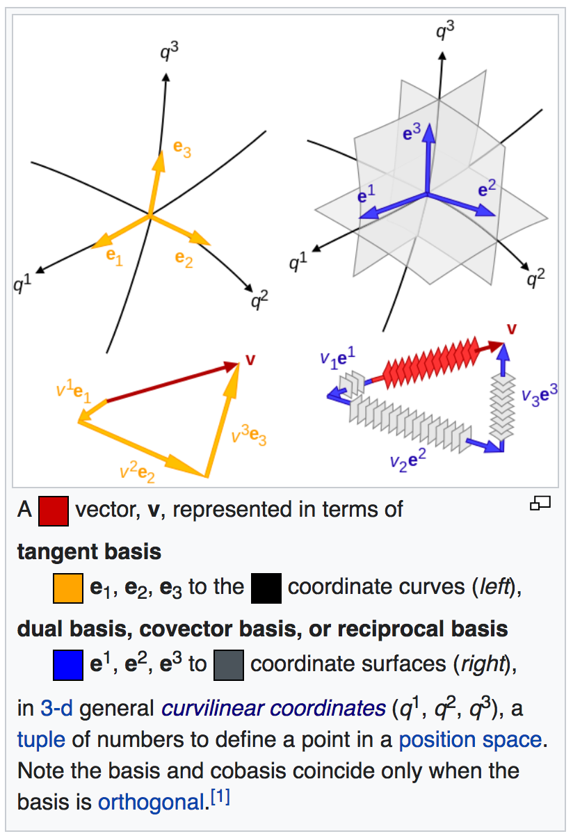
Duality
\, v_1 \, v_2 \,v_3 \, ,
\, v^1 \, v^2 \, v^3 \, ,
\, e_1 \, e_2 \, e_3 \, ,
\, e^1 \, e^2 \, e^3 \, ,
\, e^i (e_j) = { \delta }_i^j \, ,
\, v = v^1 e_1 + v^2 e_2 + v^3 e_3 \, ,
\, [v]_E = \left< v^1, v^2, v^3 \right>_E \, ,
\, v^* = v_1 e^1 + v_2 e^2 + v_3 e^3 \, ,
\, [v^*]_{E^*} = \left< v_1, v_2, v_3 \right>_{E^*} \, .
\, v_1 = 0 \, , \, v_2 = 0 \, , \, v_3 = 0 \, .
\, v^1 = 0 \, , \, v^2 = 0 \, , \, v^3 = 0 \, .
\, v^*(v) = (v_1 e^1 + v_2 e^2 + v_3 e^3) (v^1 e_1 + v^2 e_2 + v^3 e_3) = \,
\, = v_1 v^1 \, e^1(e_1) + v_2 v^2 \, e^2(e_2) + v_3 v^3 \, e^3(e_3) = \,
\, = v_1 v^1 + v_2 v^2 + v_3 v^3 = |v_1|^2 + |v_2|^2 + |v_3|^2 = |v|^2 \, .
An analogous computation gives:
\, x^*(y) = x_1 y^1 + x_2 y^2 + x_3 y^3 \, .
///////
A vector represented in a tangent basis and its dual basis
///////

///////
The dual basis measures the size of a vector along each of its dimensions
(Ambjörn Naeve on YouTube):
The interactive simulation that created this movie
///////
The contravariant and covariant components of a vector
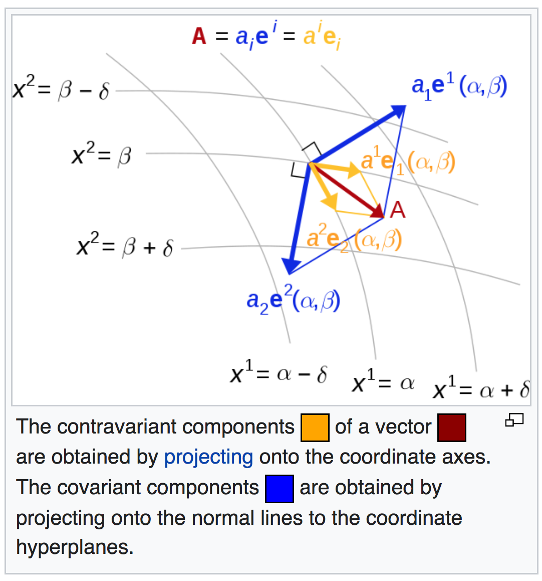
///////
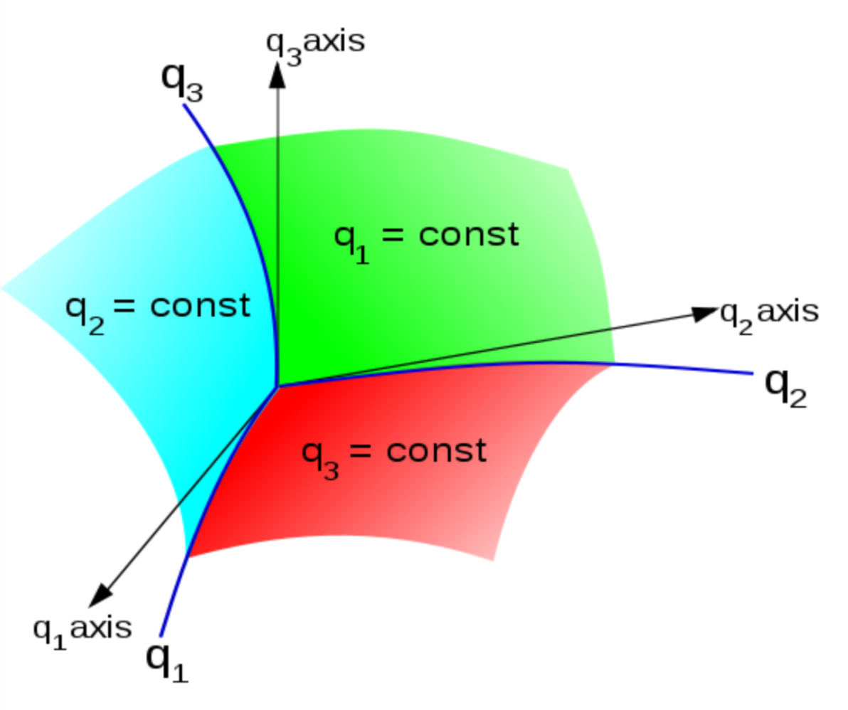
Basis and dual basis in a curvilinear coordinate system (Wikipedia)
///////
1-tensor = ∑ (basisvector cocoordinate) = ∑ (basiscovector coordinate)
///////
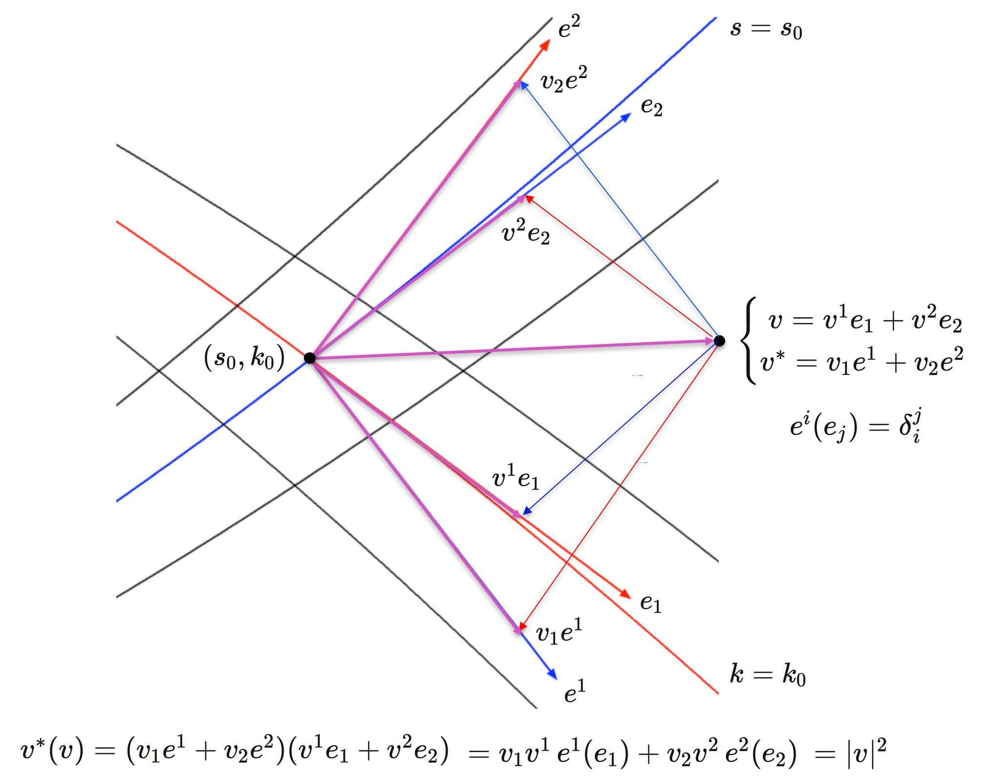
The coordinate curves intersect at the point
\, (s_0, k_0) \,\, s = s_0 \, k = k_0 \, ,
\, e^1 \,\, e^2 \, ,
\, e^i (e_j) = { \delta }_i^j \, ,
\, v = v_1 e^1 + v_2 e^2 \, .
\, v = v^1 e_1 + v^2 e_2 \, .
\, \begin{cases} \; v = v^1 e_1 + v^2 e_2 \\ v^* = v_1 e^1 + v_2 e^2 \end{cases} \, .
\, v^*(v) = (v_1 e^1 + v_2 e^2) (v^1 e_1 + v^2 e_2) = \,
\, = v_1 v^1 \, e^1(e_1) + v_2 v^2 \, e^2(e_2) = \,
\, = v_1 v^1 + v_2 v^2 = |v_1|^2 + |v_2|^2 = |v|^2 \, .
///////
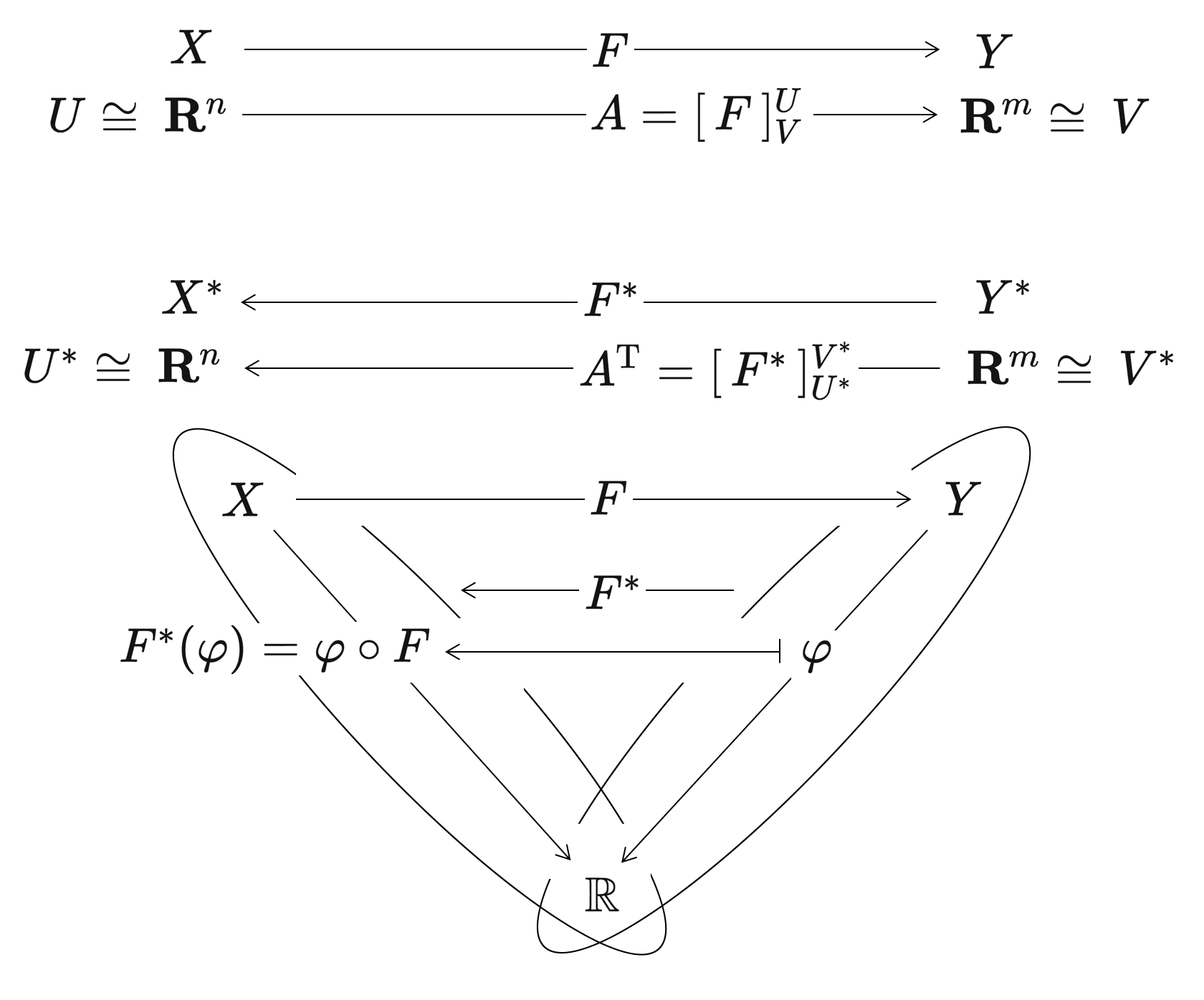
Linear transformations F and F* with matrices A and A^T
(x_1, x_2, \cdots, x_n) \begin{pmatrix} x_1 \\ x_2 \\ \vdots \\ x_n \end{pmatrix} \, = \, x_1^2 + x_2^2 + \cdots + x_n^2 \, .
(x^1, x^2, \cdots, x^n) \begin{pmatrix} x_1 \\ x_2 \\ \vdots \\ x_n \end{pmatrix} \, = \, x^1 x_1 + x^2 x_2 + \cdots + x^n x_n \, .
///////