This is a sub-page of our page on Infinitesimal Calculus of One Real Variable.
///////
Related KMR pages:
• Integration in One Real Variable
///////
Other relevant sources of information:
• The fundamental theorem of calculus
• The Riemann integral
• The Riemann-Stiltjes integral
• The Lebesgue integral
• The Lebesgue-Stiltjes integral
• Measure
• The gauge integral
///////
The interactive simulations on this page can be navigated with the Free Viewer
of the Graphing Calculator.
///////
A list of anchors into the text below:
• The essence of calculus
• Integration and the fundamental theorem of calculus
• What does area have to do with slope?
• Integration and the fundamental theorem of calculus | Essence of calculus, chapter 8
• A Wikimedia animation of the fundamental theorem of calculus
• Content of the fundamental theorem of calculus
• To differentiate a function means to compute its derivative
• History of the fundamental theorem of calculus
• The Leibniz-Newton calculus controversy
• How Newton’s calculus revolutionised the computation of π
• Classical contributions to infinitesimal calculus
• Stokes theorem
• Generalized Stokes theorem
• Recapturing the fundamental theorem
• Some applications of the fundamental theorem of calculus
• The chain rule
///////
The essence of calculus (3Blue1Brown on YouTube):
///
Integration and the fundamental theorem of calculus (3Blue1Brown on YouTube):
///
What does area have to do with slope? (3Blue1Brown on YouTube):
///
Integration and the fundamental theorem of calculus | Essence of calculus, chapter 8 (3Blue1Brown on YouTube):
/////// Quoting Wikipedia on the “Fundamental theorem of calculus”:
The fundamental theorem of calculus is a theorem that links the concept of differentiating a function with the concept of integrating a function.
The first part of the theorem, sometimes called the first fundamental theorem of calculus, states that one of the antiderivatives (also called indefinite integrals), say \, F , of some function \, f \, may be obtained as the integral of \, f \, with a variable bound of integration. This implies the existence of antiderivatives for continuous functions.[1]
Conversely, the second part of the theorem, sometimes called the second fundamental theorem of calculus, states that the definite integral of a function \, f \, over some interval can be computed by using any one, say \, F , of its infinitely many antiderivatives. This part of the theorem has key practical applications, because explicitly finding the antiderivative of a function by symbolic integration avoids numerical integration to compute integrals. This provides generally a better numerical accuracy.
///////
A Wikimedia animation of the fundamental theorem of calculus


///////
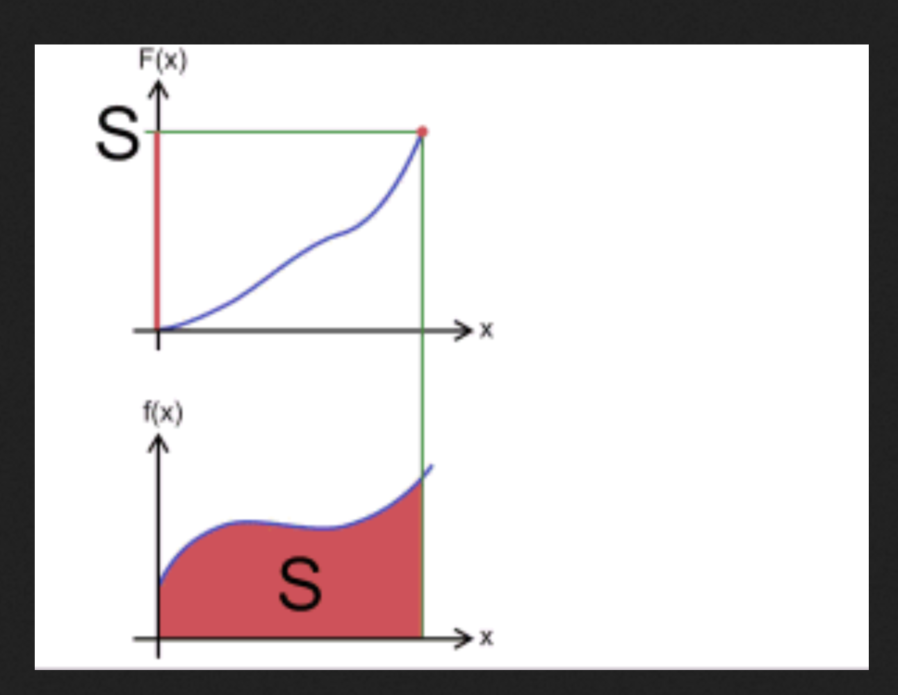
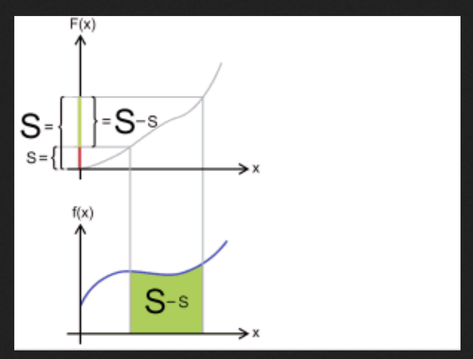
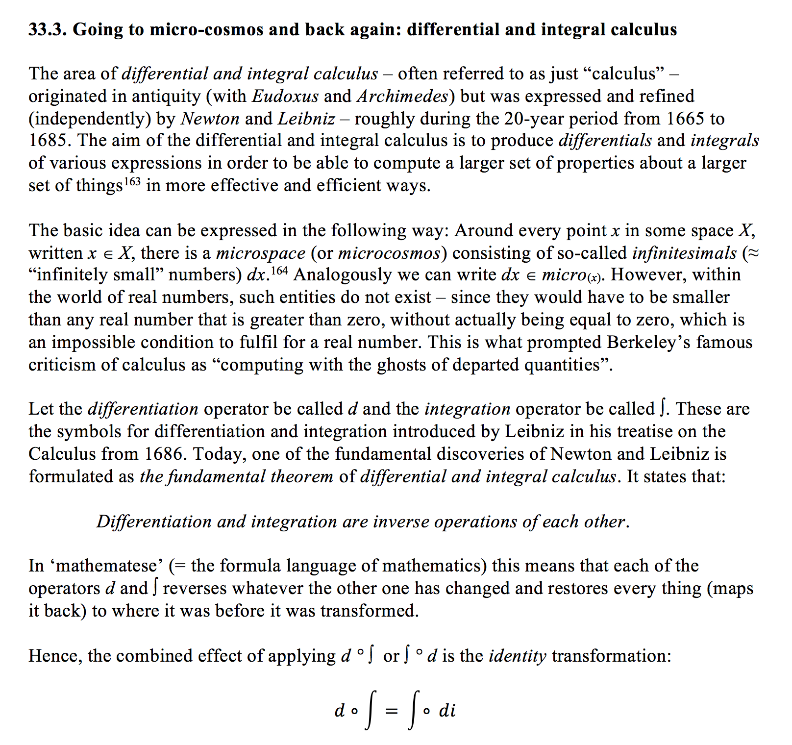
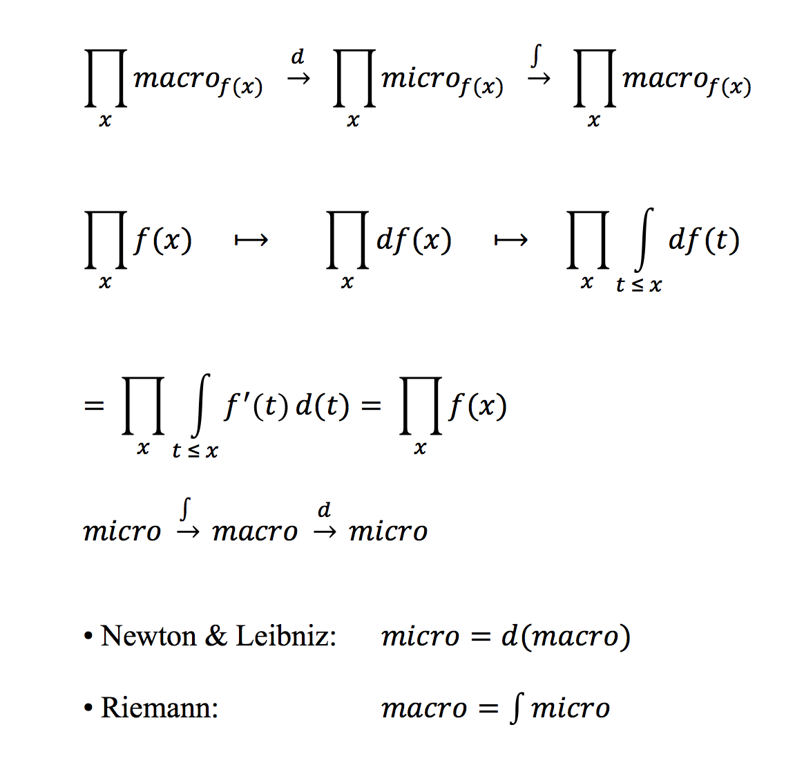
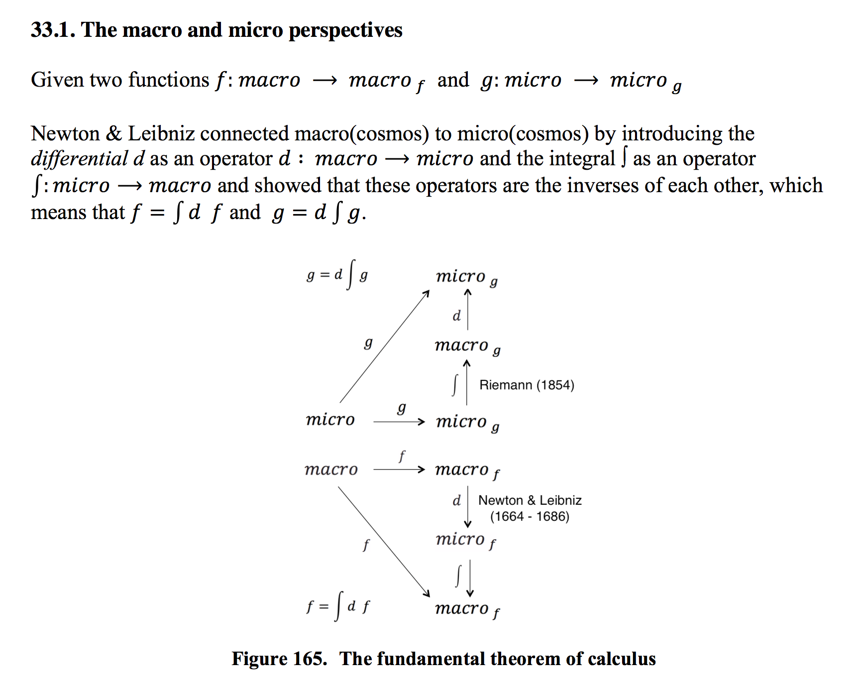
Content of the fundamental theorem of calculus:
A sufficiently ‘well-behaved’ function can be expressed both as
the integral of its differential, and as
the derivative of its integral.
More precisely expressed:
The value of a differentiable function, (i.e., a function that has a derivative)
at some specific point can be expressed as:
(1): the integral of the function’s differential
over the interval that lies to the left of this point.
(2): the derivative at this point of the function’s integral
over the interval that lies to the left of this point.
NOTE: In order for (2) to be valid it is only necessary that the function is continuous,
since its integral in this case automatically becomes differentiable,
i.e., it automatically has a derivative.
In “mathematese” one can express the fundamental theorem like this:
(if the function is called \, f \, and the examined point is called \, x ):
(1): \, f(x) \, \equiv \, \int_{}^{x} df \, \equiv \, {{\int} \atop {u \, \leq \, x}} \, df(u) \, \equiv \, {{\int} \atop {u \, \leq \, x}} \, f'(u) \, du \, ,
(2): \, f(x) \equiv \, \frac{d}{dx} \, ( \int_{}^{x} f ) \, \equiv \, \frac{d}{dx} \, ( \, {{\int} \atop {u \, \leq \, x}} \, f(u) du \, ) \, \equiv \,
\;\;\;\;\;\;\;\;\;\;\;\;\; \equiv \, \frac{d}{dx} \, ( {{\int} \atop {u(v) \,\, \leq \, x}} \, f(u(v)) \, u'(v) dv ) .
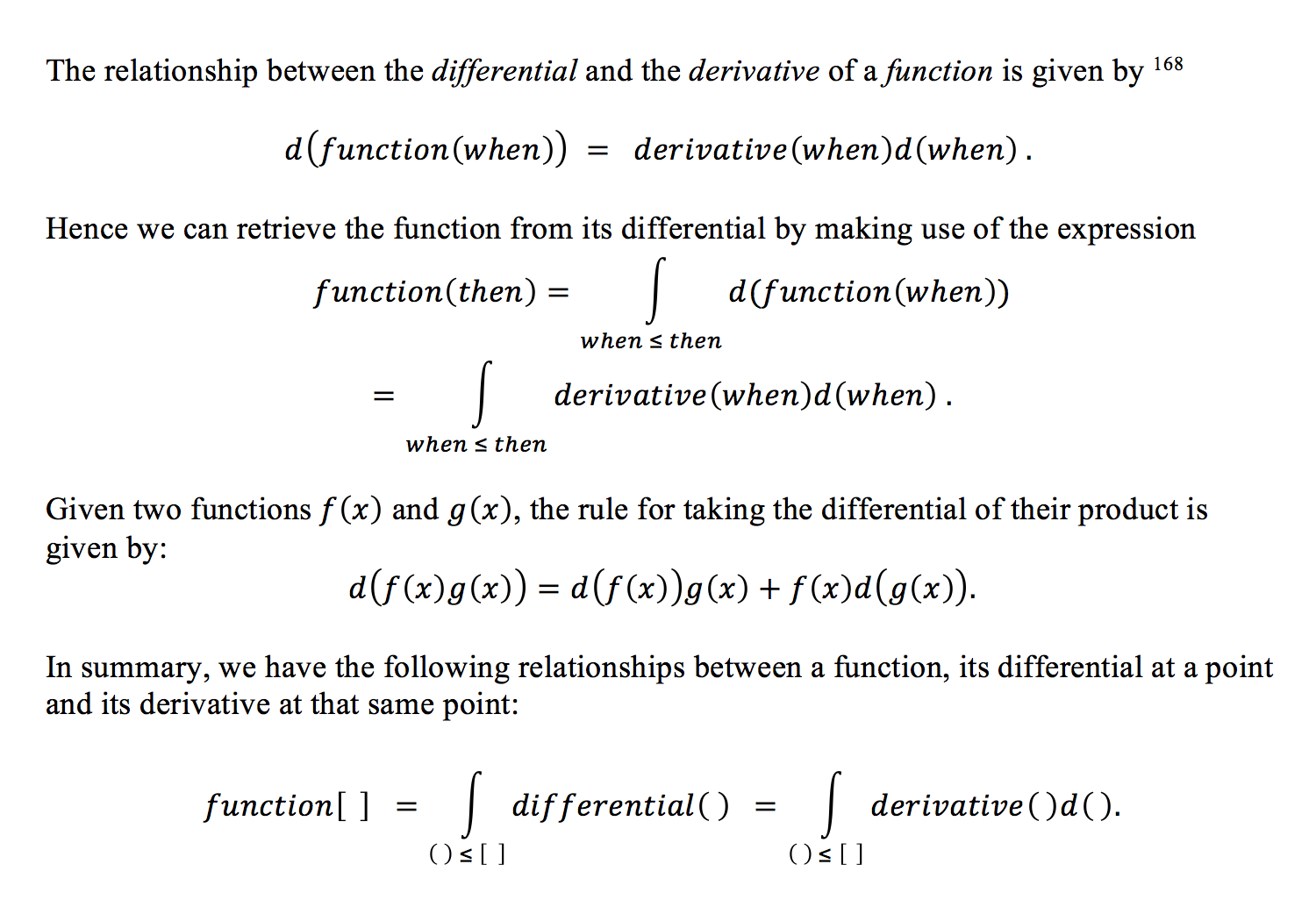
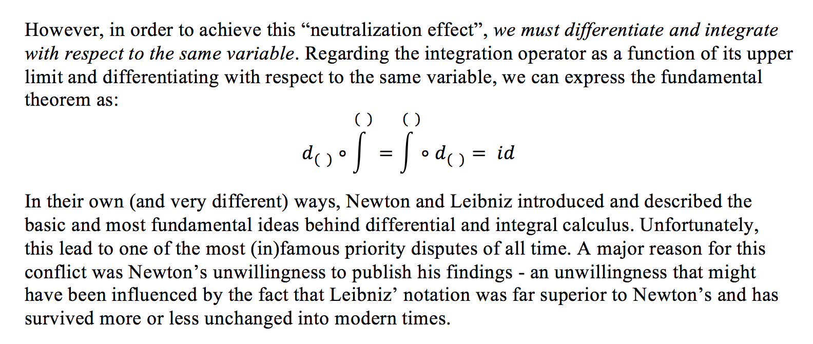
In fact it is only the first equalities in (1) and (2) above that express the actual fundamental theorem , i.e., that a function can be expressed both as the integral of its differential and as the derivative of its integral.
The rest of the equalities in (1) och (2) describe the behavior of these expressions under a
To differentiate a function means to compute its derivative
NOTE: For reasons of conceptual clarity we recall the linguistic incongruity of English within this context:
When we differentiate a function
we are in fact computing the function’s derivative.
/////// In Swedish:
På svenska gör vi ofta misstaget att följa den engelska terminologin i stället för att utnyttja svenskans möjligheter till språklig kongruens genom att kalla den process som producerar en “derivata” för “derivering.”
Att derivera en funktion är alltså en operation vars resultat är funktionens derivata.
Tyvärr har alltså denna operation på engelska den missvisande beskrivningen “to differentiate a function.”
Därför är det högst förståeligt att begreppen differential och derivata ofta blandas ihop med varandra. På engelska betyder som sagt verbet differentiate (i matematisk mening) att beräkna derivatan av en funktion. Denna språkliga inkongruens beror på att termen “derive” har en helt annan betydelse på engelska än den som termen “derivera” har på svenska.
NOTERA: Det är värt att notera att Wiktionary INTE har blandat ihop begreppen.
Där beskrivs korrekt: att differentiera en funktion betyder att beräkna dess differential.
Resultatet av en derivering, dvs derivatan kallas lutning eller förändringshastighet i det endimensionella fallet och matrisderivata, totalderivata, Fréchetderivata, funktionalmatris eller Jacobimatris i det flerdimensionella fallet.
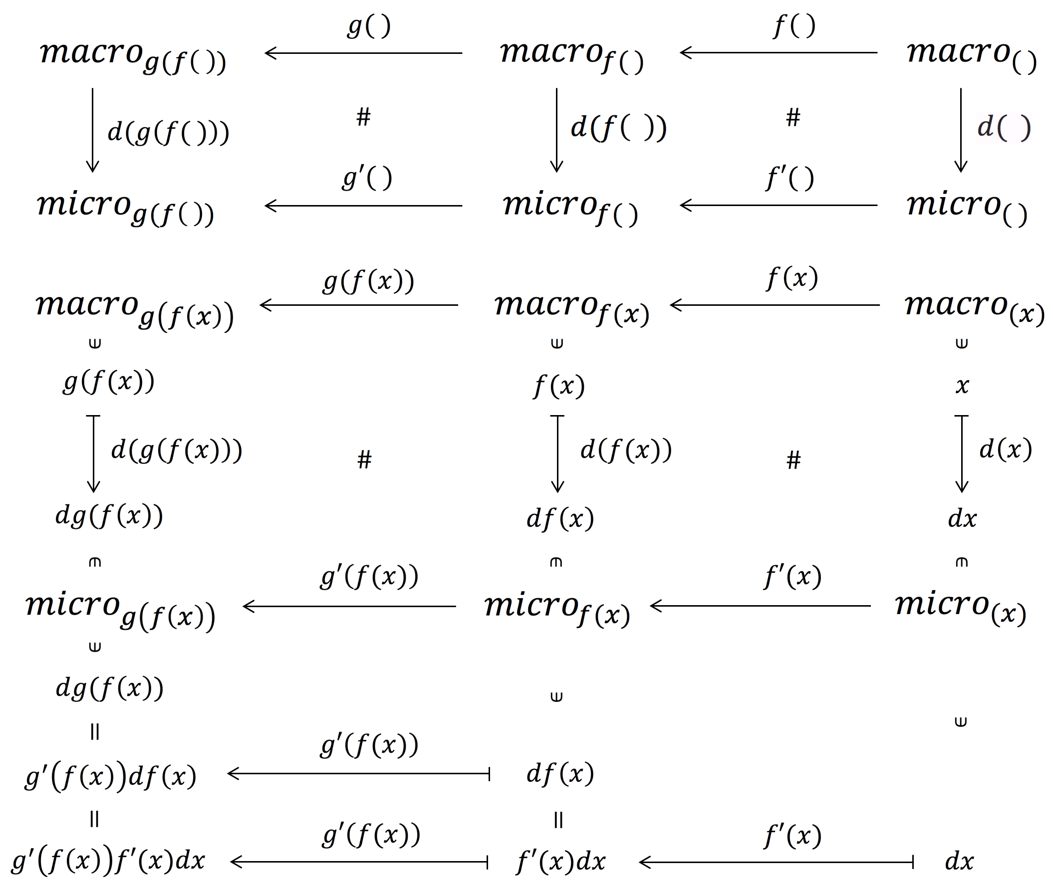
Att differentiera och derivera länkarna i en sammansättningskedja av funktioner
resulterar i den s.k. kedjeregeln (the chain rule) – en av infinitesimalkalkylens viktigaste räknelagar:
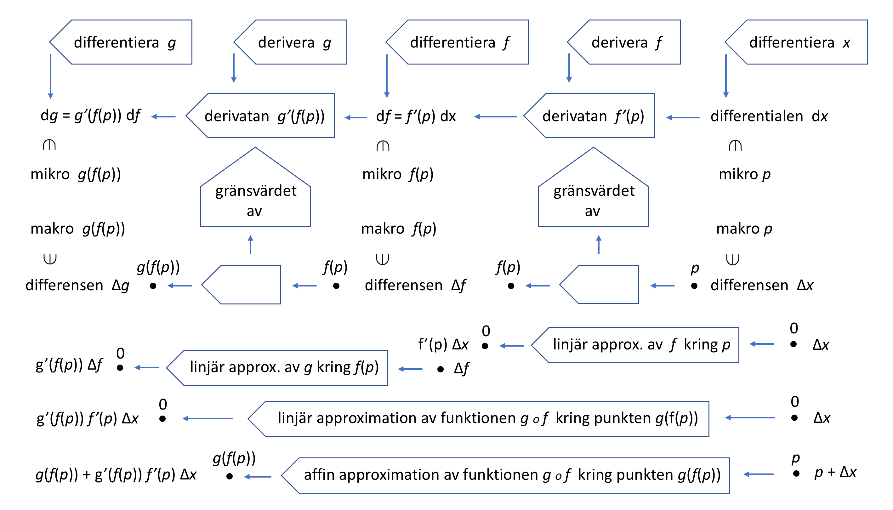
Ovanstående begreppsanalys visar att det är svårt att beskriva skillanderna mellan begreppen “differential” och “derivata” på ett formelfritt sätt.
/////// English below:
History of the fundamental theorem of calculus
The fundamental theorem of calculus was formulated and proved for the first time (for the special case of monotone functions) by James Gregory (1638–1675) in his book Geometriae Pars Universalis from 1668. Isaac Barrow (1630–1677) extended the theorem to a larger class of functions and his student Isaac Newton (1642–1727) completed the development of the underlying theory and methodology of the emerging infinitesimal calculus. Newton wrote down his ideas in a manuscript which he called the Method of Fluxions. The manuscript was completed in 1671, but it was not published until 1736 – almost ten years after Newton’s death.
Independently of Newton, Gottfried Wilhelm von Leibniz (1646–1716) developed his own version of the infinitesimal calculus, which included a very clever notation which, in its essentials, has remained in use ever since.
The Leibniz-Newton calculus controversy
/////// Quoting Wikipedia
The calculus controversy (German: Prioritätsstreit, “priority dispute”) was an argument between the mathematicians Isaac Newton and Gottfried Wilhelm Leibniz over who had first invented calculus. The question was a major intellectual controversy, which began simmering in 1699 and broke out in full force in 1711. Leibniz had published his work first, but Newton’s supporters accused Leibniz of plagiarizing Newton’s unpublished ideas.
Leibniz died in disfavor in 1716 after his patron, the Elector Georg Ludwig of Hanover, became King George I of Great Britain in 1714. The modern consensus is that the two men developed their ideas independently.
/////// End of Quote from Wikipedia
Newton‘s version of the infinitesimal calculus was in fact based on expanding a function in a type of power series later known as Taylor series or, when expanding around the origin, as MacLaurin series.
Newton arrived at his method by generalizing the binomial theorem – which is about expanding \, (a + b)^n \, – to non-integer (= fractional and real) exponents, such as e.g. \, (a + b)^{1/2} . This extension, which turns the binary polynomial into an infinite series, took place during the ”miraculous years” 1664-1666 when the University of Cambridge was closed because of the plague.
Through his method of series expansion – which Newton called the Method of Fluxions – he was able to differentiate and integrate any function that could be expanded in a power series – by differentiating respectively integrating its Taylor series term by term.
Newton’s approach made it difficult for him to present his results within the framework of the calculus of series expansion by which he had arrived at them. He therefore translated the path-breaking results of his fundamental work in newtonian mechanics – Philosophiae Naturalis – Principia Mathematica from 1687 – into synthetic geometry in the style of Euclid’s Elements, which resulted in a lot of curious mathematical relationships that involved ellipses, parabolas and hyperbolas.
In essence, Newton ”covered his tracks of discovery” and could therfore never bring himself to publish anything in a style that he wasn’t satisfied with regarding the mathematics behind his ”Principia”.
Leibniz, in contrast, developed a superb notation which is still in use, and when he published his version of the infinitesimal calculus in the book Nova Methodus pro Maximis et Minimis in 1684 this came as a chock to Newton.
Newton had described his method in a manuscript from 1671: The Method of Fluxions and Infinite Series: With Its Application to the Geometry of Curve-lines, but this was not published until 1736, almost ten years after Newton’s death.
///////
How Newton’s calculus revolutionised the computation of π ( Veritasium on YouTube):
///////
Classical contributions to infinitesimal calculus
Eudoxus
Eudoxus of Cnidus (408 – c. 355 BC) is commonly regarded as the second-greatest mathematician of antiquity, second only to Archimedes. Eudoxus made important contributions to the theory of proportion, where he made a definition allowing possibly irrational lengths to be compared in a similar way to the method of cross-multiplication used today.
The theory developed by Eudoxus is set out in Euclid’s Elements. Definition 4 in that Book is called the Axiom of Eudoxus and was attributed to him by Archimedes.
It is difficult to exaggerate the significance of the theory of proportion, because it amounts to a rigorous definition of real number. Number theory was allowed to advance again, after the paralysis imposed on it by the pythagorean discovery of irrationals.
Another remarkable contribution to mathematics made by Eudoxus was his early work on integration using his method of exhaustion. This work developed directly out of his work on the theory of proportion since he was now able to compare irrational numbers.
Archimedes
Archimedes of Syracuse (c. 287 – c. 212 BC) is commonly regarded as the greatest mathematician of antiquity and made fundamental contributions to many fields of mathematics and physics.
His contributions to integral calculus were revealed in 1906, when an important manuscript of Archimedes called The Method of Mechanical Theorems was recovered as a so-called Palimpsest – known as the Archimedes’ palimpsest.
A palimpsest is is a manuscript page, either from a scroll or a book, from which the text has been scraped or washed off so that the page could be reused for another document. The complex manuscript of Archimedes was not appreciated by the medieval monks at the remote monastery where it ended up, and it was soon overwritten (1229 AD) with a religious text.
///////
Two generalizations of the fundamental theorem
Stokes theorem
Within vector analysis there is a generalisation of the fundamental theorem of calculus which is called Stokes theorem. It says that the surface integral of the rotation of a vector field \, F \, over a surface in Euclidean space is equal to the line integral of the vector field \, F \, over the boundary curve of the surface.
Generalized Stokes theorem
Within differential geometry there is a generalization of Stokes theorem that is called the generalized Stokes theorem. It deals with integration of differential forms over manifolds. The generalized Stokes theorem both simplifies and generalizes a number of different theorems within the field of vector analysis
The generalized Stokes theorem says that the integral of a differential form \, \omega \, over the boundary of an orientable manifold \, \Omega \, is equal to the integral of its exterior derivative \, d \omega \, over the whole of \, \Omega , that is:
\, \int\limits_{\partial \Omega}^{ } \omega \, \equiv \, \int\limits_{\Omega}^{ } d \omega .
An interesting visual representation of differential forms (including exterior derivatives)
can be downloaded from here.
On a differentiable manifold, the exterior derivative extends the concept of the differential of a function to differential forms of higher order.
/////// Connect with De Rham cohomology
A great advantage of this level of abstraction is that it does not depend on dimension. In many common applications the domain of integration \, \Omega \, is an \, n -dimensional region
and \, \partial \Omega \, is its \, (n-1) -dimensional boundary.
Recapturing the fundamental theorem
By applying the generalized Stokes theorem to integrals over one-dimensional real-valued functions, where the boundary of an interval is the formal difference of its two endpoints, i.e., \, \partial [a, b] = b - a \, , we arrive at the fundamental theorem of infinitesimal calculus.
Let \, F \, be a so-called primitive function (= antiderivative = indefinite integral) of the function f . By definition this means that \, F' \equiv f .
The integral of a function \, f \, over an interval \, [a, b] \, is equal to
the integral of the function \, F \, over the boundary of the interval \, [a, b] .
Since we know that this boundary is equal to \, b - a \, we arrive at:
\, \int\limits_{a}^{b} f(x)dx \, = \, \int\limits_{\partial [a, b]}^{ } F \, = \, F(b) - F(a) .
For a differentiable function \, f \, we can therefore formulate the fundamental theorem like this:
\, \int\limits_{a}^{b} f'(x)dx \, \equiv \, \int\limits_{[a, b]}^{ } df \, \equiv \int\limits_{\partial [a, b]}^{ } f \, \equiv \, f(b) - f(a) \, .
///////
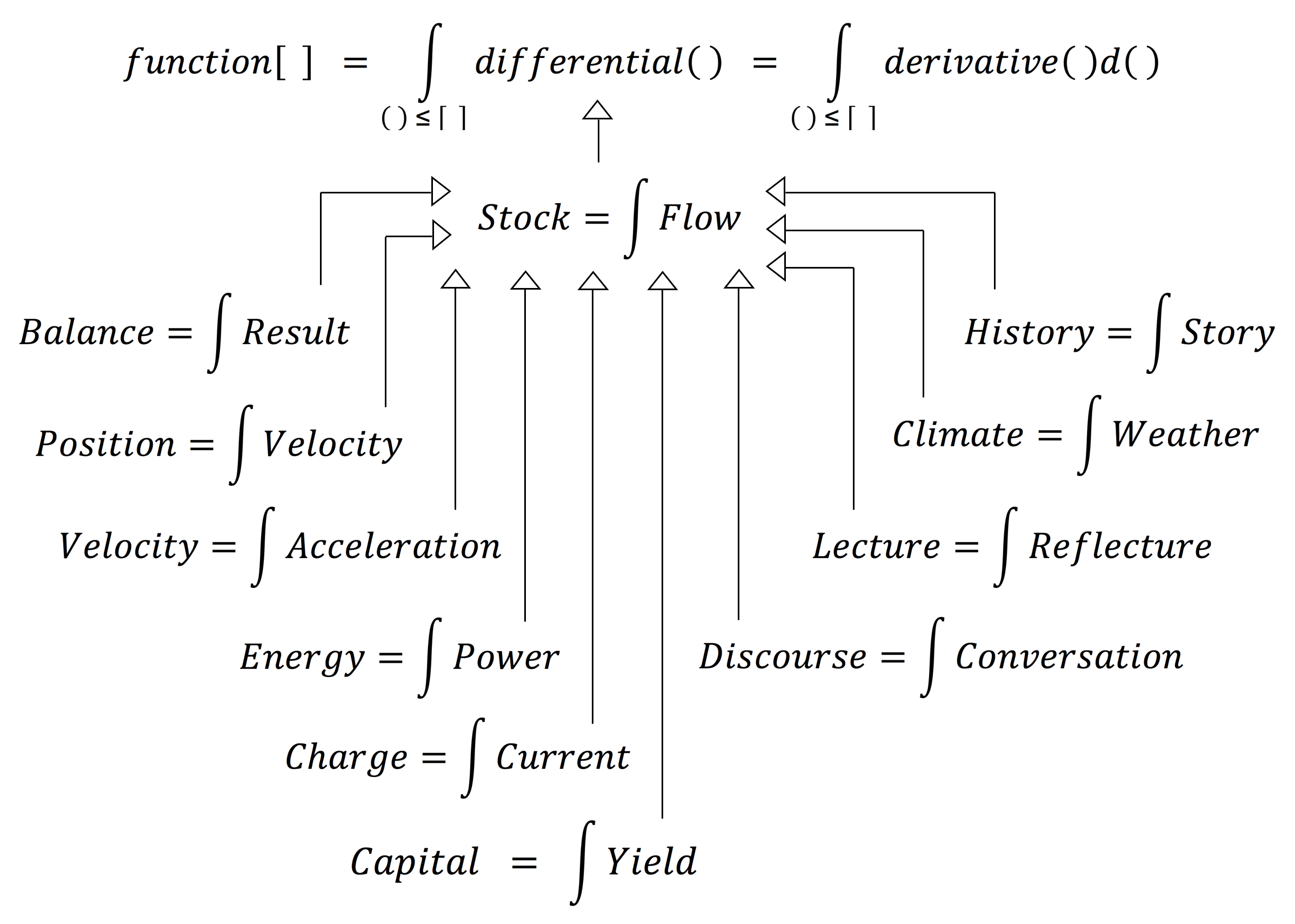
Some applications of the fundamental theorem of calculus:
///////
///////

///////

///////
///////
The chain rule:
///////

///////
///////
///////
///////

///////

///////
///////
///////
///////