This is a sub-page of our page on Geometric Algebra.
///////
The sub-pages of this page are:
///////
Related KMR-pages:
• Geometric Numbers in Euclidean 3D-space
• Clifford Algebra
• Geometric Algebra
• Quaternions
• Disambiguating plus – learning to add and multiply apples and pears
• Dimension
///////
Other relevant sources of information:
• Oliver Heaviside – The Life, Work, And Times Of An Electrical Genius Of The Victorian Age, by Paul J. Nahin, The Johns Hopkins University Press, 2002 (1987).
///////
The interactive simulations on this page can be navigated with the Free Viewer
of the Graphing Calculator.
///////
Representation: \, [ \, p_{resentant} \, ]_{B_{ackground}} \, = \, \left< \, r_{epresentant} \, \right>_{B_{ackground}}
///////
Geometric numbers on the real line:
\, [ \, G_{eometric}N_{umber} \, ]_{\mathbb{R}} = \left< \, r_{adius} \, \right>_{\mathbb{R}} .
The \, r_{adius} , which can be negative, expresses the amount of directed expansion.
Multiplication: \, {\left< \, r_{adius} \, \right>}_{1 * 2} \, = \, { \left< \, {r_{adius}}_1 * {r_{adius}}_2 \, \right> }_{1 * 2} .
/////// Stubs:
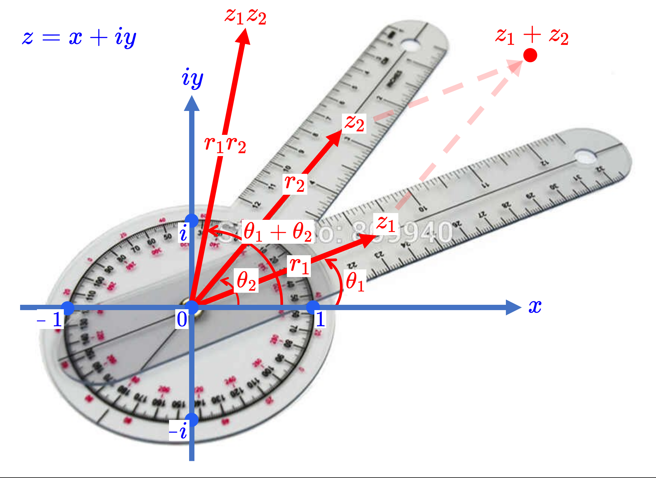
\, \textcolor{blue} { \, -i \, -1 \, 1 \, 0 \, z = x + i \, y } \,
\, \textcolor{red} {z_1 = r_1 e^{i \, {\theta}_1}} \,
\, \textcolor{red} {z_2 = r_2 e^{i \, {\theta}_2}} \,
\, \textcolor{red} {z_1 z_2 = r_1 r_2 \, e^{i ( \, {\theta}_1 + \, {\theta}_2 \, ) }} \,
\, \textcolor{red} {z_1 + z_2} \,
\, \textcolor{red} { {\theta}_1 \, , \, {\theta}_2 \, , \, {\theta}_1 + {\theta}_2 }
///////
\, (\cos \alpha + i \sin \alpha)(\cos \beta + i \sin \beta) = \,
\, = \, \cos \alpha \cos \beta - \sin \alpha \sin \beta + i (\sin \alpha \cos \beta + \cos \alpha \sin \beta) = \,
\, = \, \cos (\alpha + \beta) + i \sin (\alpha + \beta)
If we define
\, e^{ \, i \, \theta} \, \stackrel {\mathrm{def}}{=} \, \cos \theta + i \sin \theta ,
the product above can be written
\, e^{ \, i \, \alpha} e^{ \, i \, \beta} = e^{ \, i \, ( \alpha + \beta) }
which conforms to the usual rules of exponentiation (by transforming multiplication of two unitary rotations to addition of their respective angles).
This formula, discovered by Euler, is considered to be one of the most beautiful formulae in all of mathematics. It ties in with the transformation formulae from polar to cartesian coordinates:
\, x = r \cos \theta \, , \, y = r \sin \theta \,
\, x + i \, y = r \cos \theta + i \, r \sin \theta = r (\cos \theta + i \, \sin \theta) = r e^{ \, i \theta}
//////////////////////////////////////////////////////
Geometric numbers in the Euclidean plane:
\, [ \, G_{eometric}N_{umber} \, ]_{\text{Polar} \, \mathbb{R}^2} \, = \, \left< \, r_{adius}, a_{ngle} \, \right>_{\text{Polar} \, \mathbb{R}^2}
The \, r_{adius} \, expresses the amount of directed expansion
and the \, a_{ngle} \, expresses the amount of directed rotation
contained in the \, G_{eometric}N_{umber} .
Multiplication: \, {\left< \, {r_{adius}, a_{ngle}} \, \right>}_{1 * 2} \, = \, {\left< \, {r_{adius}}_1 * {r_{adius}}_2 \, , {a_{ngle}}_1 + {a_{ngle}}_2\, \right>}_{1 * 2}
Combining multiplications:
\, [ \, q_{uarter}T_{urn} * q_{uarter}T_{urn} \, ]_{\mathbb{R}^2} \, = \, [ \, q_{uarter}^2T_{urn} \, ]_{\mathbb{R}^2} = \, [ \, h_{alf}T_{urn} \, ]_{\mathbb{R}^2} \, = \, - [ \, z_{ero}T_{urn} \, ]_{\mathbb{R}^2}
\, \textcolor{red}{q_{uarter}T_{urn}}(\textcolor{blue}{q_{uarter}T_{urn}}(s_{tart})) \, = \, q_{uarter}^2T_{urn}(s_{tart}) = h_{alf}T_{urn}(s_{tart}) = - s_{tart} = (-1) s_{tart}
Hence, for this multiplicative algebra to work, we must have \, q_{uarter}^2T_{urn} = -1 .
Cartesian coordinate system:
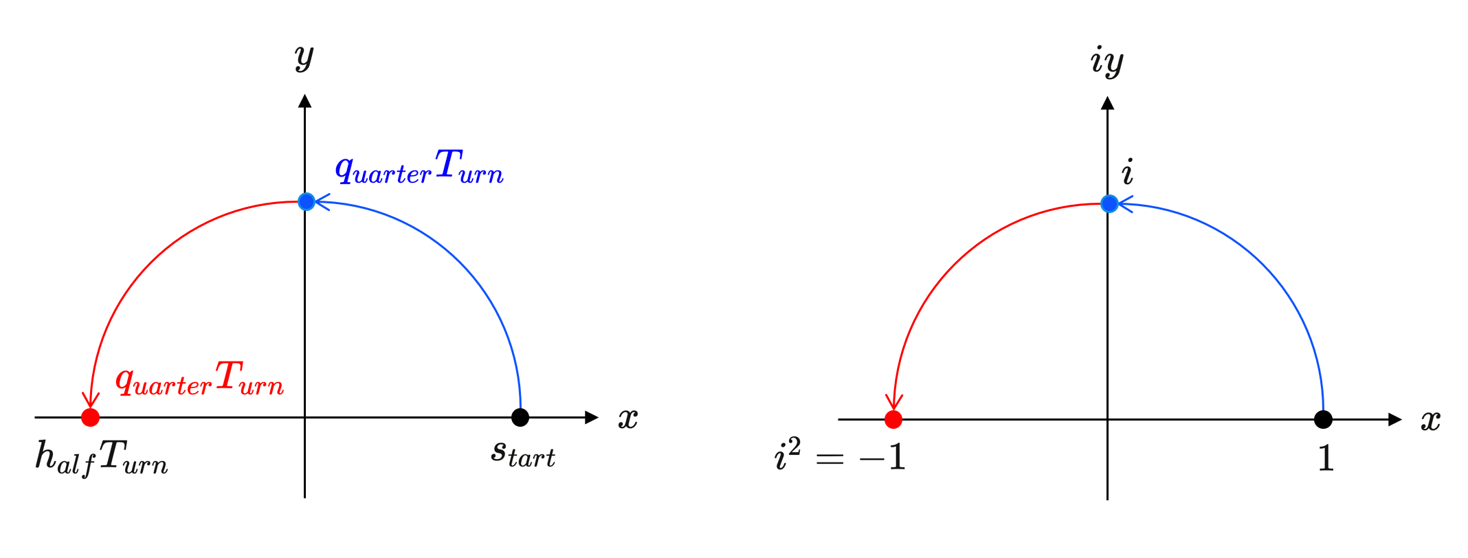
\, i^2 = -1 \,
\, [ \, G_{eometric}N_{umber} \, ]_{\text{Cartesian} \, \mathbb{R}^2} \, = \, \left< \, x + iy \, \right>_{\text{Cartesian} \, \mathbb{R}^2}
Addition:
\, \left< \, (x_1 + i y_1) + (x_2 + i y_2) \, \right>_{\text{Cartesian} \, \mathbb{R}^2} \, = \, \left< \, (x_1 + x_2) + i (y_1 + y_2) \, \right>_{\text{Cartesian} \, \mathbb{R}^2}
Multiplication:
Since we work with numbers, we want distributivity of \, * \, over \, + \, , and therefore we can aim for this:
\, \left< \, (x_1 + i y_1) * (x_2 + i y_2) \, \right>_{\text{Cartesian} \, \mathbb{R}^2} \, =
\, = \, \left< \, (x_1 x_2 + x_1 i y_2) + i y_1 x_2 + i y_1 i y_2) \, \right>_{\text{Cartesian} \, \mathbb{R}^2} \, =
\, = \, \left< \, (x_1 x_2 - y_1 y_2) + i (x_1 y_2 + x_2 y_1) \, \right>_{\text{Cartesian} \, \mathbb{R}^2}
An important question is now whether or not this multiplication of geometric vectors in Cartesian \mathbb{R}^2 \, is compatible with (= equivalent to) the multiplication defined above for geometric vectors in Polar \mathbb{R}^2 . If not, we are not building a coherent mathematical representation of geometric vectors.
////////////////////////////////////////////////////
Geometric numbers in the complex plane:
Representations of multiplication:
\, [ \, z_1 \, z_2 \, ]_{R_{ectangular}} \, = \, \left< \, (x_1 + i y_1) \,(x_2 + i y_2) \,\right>_{R_{ectangular}} \, = \,
\,\;\;\;\;\;\;\;\;\;\;\;\;\;\;\;\;\;\;\;\;\;\; \, = \left< \, (x_1 x_2 - y_1 y_2) + i (x_1 y_2 + x_2 y_1) \, \right>_{R_{ectangular}} \,
\, [ \, z_1 \, z_2 \, ]_{P_{olar}} = \, \left< \, r_1 e^{i {\theta}_1} \, r_2 e^{i {\theta}_2} \, \right>_{P_{olar}} \, = \,
\, \;\;\;\;\;\;\;\;\;\;\;\;\;\;\;\; = \, \left< \, r_1 r_2 e^{i({\theta}_1 + \, {\theta}_2)} \, \right>_{P_{olar}} \,
Animation of complex multiplication with filled triangles:
Interactive simulation of the multiplication of complex numbers.
///// This link has to be updated: More interactive simulations on basic arithmetic with complex numbers.
///////////////////////////////////////////////////////////////////////////
The complex numbers represented as the even subalgebra
of the clifford algebra \, C_l(e_1, e_2) \, over the real numbers \, \mathbb{R} :
\, e_1, e_2 \,
\, e_1^2 = e_2^2 = 1 \,
\, e_2 e_1 = - e_1 e_2 \,
Hence we have: \, (e_1 e_2)^2 = e_1 e_2 e_1 e_2 = - e_2 e_1 e_1 e_2 = - e_2 e_2 = -1 –
\, \alpha_1 e_1 + \alpha_2 e_2 \,
\, \alpha'_1 e_1 + \alpha'_2 e_2 \,
\, (\alpha_1 e_1 + \alpha_2 e_2) (\alpha'_1 e_1 + \alpha'_2 e_2) =
\, = \alpha_1 e_1 \alpha'_1 e_1 + \alpha_1 e_1 \alpha'_2 e_2 + \alpha_2 e_2 \alpha'_1 e_1 + \alpha_2 e_2 \alpha'_2 e_2 \, =
= \, \alpha_1 \alpha'_1 e_1 e_1 + \alpha_2 \alpha'_2 e_2 e_2 + \alpha_1 \alpha'_2 e_1 e_2 + \alpha_2 \alpha'_1 e_2 e_1 \, =
= \, \alpha_1 \alpha'_1 + \alpha_2 \alpha'_2 + \alpha_1 \alpha'_2 e_1 e_2 - \alpha_2 \alpha'_1 e_1 e_2 \, =
= \, \alpha_1 \alpha'_1 + \alpha_2 \alpha'_2 + (\alpha_1 \alpha'_2 - \alpha_2 \alpha'_1) e_1 e_2 .
/////// The even part of the clifford algebra \, C_l(e_1, e_2) \, :
\, (x + y e_1 e_2) (x' + y' e_1 e_2) \, =
= \, x x' + x y' e_1 e_2 + y e_1 e_2 x' + y e_1 e_2 y' e_1 e_2 \, =
= \, x x' + x y' e_1 e_2 + y x' e_1 e_2 + y y' e_1 e_2 e_1 e_2 \, =
= \, x x' + x y' e_1 e_2 + y x' e_1 e_2 - y y' e_2 e_1 e_1 e_2 \, =
= \, x x' - y y' + (x y' + y x') e_1 e_2 .
/////// Multiplication of complex numbers:
\, (x + iy ) (x' + iy') \, =
= \, x x' + i x y' + i y x' + i^2 y y' \, =
= \, (x x' - y y') + i (x y' + y x') .
///////
/////// Quoting Nahin (2002, p. 204):
TECH NOTE 1: NUMBERS AND VECTORS – REAL, COMPLEX, AND HYPERCOMPLEX
When mathematicians broke free of the constraints of the infinite real line, and it was realized that a vastly richer system of numbers, the so-called complex numbers (a term due to the great mathematician C. F. Gauss), could be associated with the points of the infinite plane, an enormous intellectual step was taken. It is virtually impossible to exaggerate the importance of this step. Today’s electrical engineers and physicists would be paralyzed if their beloved square root of minus one were to be taken away from them, and many other scientists would be reduced to a nearly miserable state, as well.
Think geometrically. If we associate numbers with the points along a horizontal line (the real axis), then, even though this line goes to infinity in both directions, we still imagine we know its “middle,” which we agree to call the origin, and define a vector as the directed line segment from the origin to one of the points. We can transform such a vector into another by multiplying by the appropriate number , e.g., \, +2 \, transforms into \, -2 \, when multiplied by \, -1 .
Multiplication by a positive number can be thought of as merely a contraction (or expansion). Multiplication by a negative number, however, has a more exotic interpretation, that of rotation. When we multiply \, +2 \, by \, -1 \, we rotate the \, +2 \, vector through 180˚ so that it is then pointing down the negative real axis toward \, -2 . The idea of rotation is the breakthrough concept, because it gives us a geometric interpretation of the invaluable \, \sqrt{-1} .
Let \, i^2 = -1 \, (and thus \, i = \sqrt{-1} . Geometrically we already know that multiplying by \, i^2 \, is equivalent to a 180˚ rotation, and since \, i^2 = i \cdot i , i.e., two successive applications of \, i \, , and since each \, i \, must have equal impact then each \, i \, must cause a 90˚ rotation! Thus is born the idea of drawing a vertical line, 90˚ from the horizontal real axis and creating the pair of axes that define the coordinates of the complex plane.
The vertical axis is often called the imaginary axis, but in fact there is nothing imaginary about it at all (it has been drawn in Fig 9.1). Although this idea seems to have been around since the late 1600s, it wasn’t until 1799 that the Norwegian Caspar Wessel specifically called the vertical axis the “axis of imaginaries.” The word imaginary is a holdover from olden times when mathematicians first stumbled upon the square root of minus one in solutions to certain algebraic equations. Not yet having a geometric interpretation for such solutions, they called them imaginary and then swept them under the rug. Even with the rotation concept, however, \, i \, has not had an easy road until comparatively recent times.
As the senior Wrangler of 1881 recalled, [68] “… it was an age when the use of \, \sqrt{-1} \, was suspect at Cambridge even in trigonometric formulae… . The imaginary \, i \, was suspiciously regarded as an untrustworthy intruder.”
To every point in the complex plane we can associate a two-dimensional vector drawn from the origin; see Fig 9.2. each such vector has a real part, \, A , and an imaginary part, \, B . It is written as \, A + iB , and, which we will see, geometrically, makes an angle \, \theta \, with the real axis. We can think of there being a unit vector pointing along the positive real axis, and another unit vector (i.e., the imaginary \, i ) pointing along the positive imaginary axis, and that an arbitrary vector can be written as a sum of multiples of these two basic unit vectors.
The length of the vector is, from the Pythagorean theorem, \, \rho = \sqrt{A^2 + B^2} , and thus \, A = \rho \cos \theta \, and \, B = \rho \sin \theta , and the vector itself is
\, A + iB = \rho (\cos \theta + i \sin \theta) .
The expression in the parenthesis is known, by Euler’s identity, to be \, e^{ \, i \, \theta} . Thus, any complex two-dimensional vector can be represented by the concise expression
\, \rho \, e^{ \, i \, \theta} \,
where \, \rho \, is length of the vector and \, \theta \, is the angle, in radians, the vector makes with the real axis. This interpretation of complex numbers has been fruitful nearly beyond words. For example, we immediately have from all this that
\, -1 = e^{ \, i \, π} \,
and from this, in turn,
\, \sqrt{-1} = i = (-1)^{1/2} = (e^{ \, i \, π})^{1/2} = e^{\, i \, π/2} .
From these results we can calculate such astonishing results as
\, \ln(-1) = i \, π
which just goes to show that you can calculate the logarithm of negative numbers (when the readout on your electronic calculator starts blinking when you try it, that’s because the designers didn’t do everything possible when they put their cirquits and algorithms inside the black box). And how about the perhaps even more astounding conclusion that
\, (\sqrt{-1})^{\sqrt{-1}} = {(e^{ \, i \, π/2})}^{ \, i} = e^{\, -π/2} = 0.2078796 .
Who would have suspected, at the beginning, that such wonderful knowledge could come from the “simple” idea of rotation!?
The idea of rotating out of a space into a new one of higher dimensionality is one that science fiction writers and their readers have really loved since the last century. If only, they speculate, “we could rotate out of our three-dimensional space of every day life, why then we would find ourselves in the fourth (or fifth, or sixth, etc.) dimension!” This wonderfully imaginative idea was dramatically used by H. G. Wells (who argued that time is the fourth dimension) in his 1895 masterpiece, The Time Machine, in his passage describing the Time Traveler‘s demonstration of a miniature time machine to his disbelieving friends:
We saw the lever turn. I am absolutely certain there was no trickery. There was a breath of wind, and the lamp flame jumped. One of the candles on the mantel was blown out, and the little machine suddenly swung around, became indistinct, was seen as a ghost for a second…and it was gone… . Then Filby said he was damned.
In his highly entertaining book Man and Time (Doubleday, 1964, pp. 122-123), J. B. Priestly gave a sequence of photographs “showing” this demonstration, faithful even to the rotation. But both Wells’ and Priestly’s images are not really correct, of course, because they describe and show the rotation taking place in three-dimensional space, itself. The actual rotation would be four dimensional, and who among the readers of this book (none more than the author) wouldn’t trade the contents of a well-stuffed safe-deposit box to learn the secret of how to perform that rotation!? Recall that in the one-dimensional space of the line we can transform a vector into another by multiplying by one number. It is obvious now that in the two-dimensional space of the plane we can transform a vector into another by multiplying by two numbers, i.e., to rotate a vector by angle \, \theta \, and multiply its length by a factor of \, \rho , multiply its complex number representation by the complex number \, \rho \, e^{ \, i \, \theta} . And then, once loose of the line and set free in the plane what, we may wonder (along with Hamilton), is to prevent it from rotating again into three-dimensional space? And shouldn’t that, conjectured Hamilton, require multiplication of a vector by three numbers to transform it into another? As it turns out, it takes four.
TECH NOTE 2: HAMILTON’S INSIGHT AT THE BROUGHAM BRIDGE
In a letter [69] to Tait, dated October 15, 1858, Hamilton wrote:
…I then felt the galvanic cirquit of thought close; and the sparks which fell from it were the fundamental equations between \, i, j, k … . I felt a problem to have been at that moment solved – an intellectual want relieved – which had haunted me for at least fifteen years before.
What Hamilton was referring to was the solution that came to him in a flash of inspiration on Monday, October 16, 1843, while walking with his wife along the Royal Canal into Dublin to attend a Council Meeting of the Royal Irish Academy. It was then he realized that it takes four (not three) numbers to accomplish a three-dimensional transformation of one vector into another. In that instant Hamilton saw that it takes one number to adjust the length, another one to specify the amount of rotation, and two more to specify the plane in which the rotation takes place.
This physical insight led Hamilton to study hypercomplex numbers with four components (or quaternions [70]) of the form
\, q = w + ix + jy + kz \,
where \, q = w, x, y , and \, z \, are ordinary real numbers and where \, i, j , and \, k \, are each an imaginary unit vector pointing in the three mutually perpendicular directions of space, in a simple extension of the “ordinary” complex numbers of two-dimensional space. The imaginaries, besides their basic property of \, i^2 = j^2 = k^2 = -1 , were defined to interact with one another (and the real number, one) as dictated by the multiplication table in Fig. 9.3, which for the first time in mathematics postulated non-commutative multiplication, e.g., \, ij = k \, while \, ji = -k . Matrix algebra shares this property, but it came after Hamilton’s quaternions.
This sort of behavior (strange, even today, to students when they first encounter a mathematical system in which commutativity fails) was motivated in Hamilton’s mind by the special requirements of rotations in three-dimensional space (as we’ll see in Tech Note 3), but he wasn’t unaware of other possible interpretations. As he wrote [71] in 1845,
Is there not an analogy between the fundamental pair of equations \, ij = k \, and \, ji = -k , and the facts of opposite currents of electricity corresponding to opposite rotations? [I presume Hamilton was thinking here of the sense of direction of the circular magnetic field around the currents.]
and later, in an 1854 letter [72] he wrote,
…Faraday may possibly remember my chat with him at Cambridge, in 1845, upon the subject of the analogy with the products of \, ijk , to the laws of electrical currents… . I sought to realize my old expectation [of developing his “electromagnetic quaternion”] today, after having translated Ampere’s law into the notation of the Calculus of Quaternions.
In a letter [73] to one of his sons (dated August 5, 1865) Hamilton wrote of that magic moment of insight when he saw all of this:
I [could not] resist the impulse – unphilosophical as it may been – to cut with a knife on a stone of the Brougham Bridge, as we passed it, the fundamental formula with the symbols \, i, j, k ; namely,
\, i^2 = j^2 = k^2 = ijk = -1
which contains the Solution of the Problem, but of course, as an inscription, has long since moldered away.
He very quickly, the very day of his discovery of quaternions, formed [74] one possible physical interpretation of what it means to add a scalar to a three-dimensional vector:
In the quaternion \, (v, x, y, z) , \, xyz \, [the vector] may determine direction and intensity; while \, v \, [the scalar] may determine the quantity of some agent such as electricity. \, x, y, z \, are electrically polarized, \, v \, electrically unpolarized… . The Calculus of Quaternions may turn out to be a Calculus of Polarities.
In his review [26] of Wilson’s vector book Heaviside had a humorous way of addressing the question of adding a vector to a scalar:
It is really quite legitimate to add together all sorts of different things. Everybody does it. My washerwoman is always doing it. She adds and subtracts all sorts of things, and performs various operations upon them (including linear operations), and at the end of the week this poor ignorant woman does an equation in multiplex algebra by equating the sum of a number of different things in the basket at the beginning of the week to a number of things she puts in the basket at the end of the week. Sometimes she makes a mistake in her operations. So do mathematicians.
/////// End of Quote from Nahin
Compare our page on Disambiguating Plus.