This page is a sub-page of our page on Matrix Algebra.
///////
The sub-pages of this page are:
• Solution of m equations in n unknowns.
///////
Related KMR pages
///////
Other related sources of information
• Strang, Gilbert (1986), Linear Algebra and its Applications, Third Edition (1988).
///////
/////// Quoting Strang (1986, p. 1):
The central problem of linear algebra is the solution of linear equations. The most important case, and the simplest, is when the number of unknowns equals the number of equations. Therefore we begin with this basic problem: \, n \, equations in \, n \, unknowns.
There are two well-established ways to solve linear equations. One is the method of elimination, in which multiples of the first equation are subtracted from the other equations – so as to remove the first unknown from those equations. This leaves a smaller system, of \, n - 1 \, equations in \, n - 1 \, unknowns. The process is repeated until there is only one equation and one unknown, which can be solved immediately. Then it is not hard to work backward, and find the other unknowns in reverse order; we shall work out an example in a moment.
A second and more sophisticated way introduces the idea of determinants. There is an exact formula called Cramer’s rule which gives the solution (the correct values of the unknowns) as a ratio of two \, n \, by \, n \, determinants. From the examples in a textbook it is not obvious which way is better ( \, n = 3 \, or \, n = 4 \, is about the upper limit on the patience of a reasonable human being).
In fact, the more sophisticated formula involving determinants is a disaster in practice, and elimination is the algorithm that is constantly used to solve large systems of equations. Our first goal is to understand this algorithm. It is generally called Gaussian elimination.
The idea is deceptively simple, and in some form it may already be familiar to the reader. But there are four aspects that lie deeper than the simple mechanics of elimination. Together with the algorithm itself, we want to explain them in this chapter. They are:
(1) the geometry of a linear equation. It is not easy to visualize a 10-dimensional plane in 11-dimensional space. It is harder to see eleven of those planes intersecting at a single point in that space – but somehow it is almost possible. With three planes in three dimensions it can certainly be done. Then linear algebra moves the problem into four dimensions, or eleven dimensions, where the intuition has to imagine the geometry (and get it right).
(2) The interpretation of elimination as a factorization of the coefficient matrix. We shall introduce matrix notation for the system of \, n \, equations, writing the unknowns as a vector \, x \, and the equations in the matrix shorthand \, A x = b . Then elimination amounts to factoring \, A \, into a product \, L U , of a lower triangular matrix \, L \, and an upper triangular matrix \, U .
First we have to introduce matrices and vectors in a systematic way, as well as the rules for their multiplication. We also define the transpose \, A^{\text{T}} and the inverse \, A^{-1} of a matrix \, A .
(3) In most cases elimination goes forward without difficulties. In some exceptional cases it will break down – either because the equations were written in the wrong order, which is easily fixed by exchanging them, or else because the equations fail to have a unique solution. In the latter case there may be no solution, or infinitely many. We want to understand how, at the time of breakdown, the elimination process identifies each of these possibilities.
(4) It is essential to have a rough count of the number of operations required to solve a system by elimination. The expense in computing often determines the accuracy in the model. The computer can do millions of operations, but not very many trillions. And already after a million steps, roundoff error can be significant. (Some problems are sensitive; others are not.) Without trying for full detail, we want to see what systems arise in practice and how they are actually solved.
The final result of this chapter will be an elimination algorithm which is about as efficient as possible. It is essentially the algorithm that is in constant use in a tremendous variety of applications. And at the same time, understanding it in terms of matrices – the coefficient matrix \, A , the matrices that carry out an elimination step or an exchange of rows, and the final triangular factors \, L \, and \, U \, – is an essential foundation for the theory.
THE GEOMETRY OF LINEAR EQUATIONS
The way to understand this subject is by example. We begin with two extremely humble equations, recognizing that you could solve them without a course in linear algebra. Nevertheless I hope you will give Gauss a chance:
\, 2 x - y = 1 \,
\, x + y = 5 .
There are two ways to look at that system, and our main point is to see them both.
The first approach concentrates on the separate equations, in other words on the rows. That is the most familiar, and in two dimensions we can do it quickly. The equation \, 2 x - y = 1 \, is represented by a straight line in the x-y plane. The line goes through the points \, x = 1, y = 1 \, , and \, x = \tfrac{1}{2}, y = 0 \, (and also through \, (0, -1) \, and \, (2, 3) \, and all intermediate points). The second equation \, x + y = 5 produces a second line (Fig. 1.1a). Its slope is \, dy/dx = -1 \, and it crosses the first line at the solution. The point of intersection is the only point on both lines, and therefore it is the only solution to both equations. It has the coordinates \, x = 2 \, and \, y = 3 \, – which will soon be found by a systematic elimination.
The second approach is not so familiar. It looks at the columns of the linear system.
The two separate equations are really one vector equation
\, x \begin{bmatrix} 2 \\ 1 \end{bmatrix} + y \begin{bmatrix} -1 \\ 1 \end{bmatrix} = \begin{bmatrix} 1 \\ 5 \end{bmatrix} .
The problem is to find the combination of the column vectors on the left side which produces the vector on the right side. Those two-dimensional vectors are represented by the bold lines in Fig. 1.1b. The unknowns are the numbers \, x \, and \, y \, which multiply the column vectors. The whole idea can be seen in that figure, where 2 times column 1 is added to 3 times column 2. Geometrically this produces a famous parallelogram. Algebraically it produces the correct vector \, \begin{bmatrix} 1 \\ 5 \end{bmatrix} , on the right side of our equations. The column picture confirms that the solution is \, x = 2, y = 3 .
More time could be spent on that example, but I would rather move forward to \, n = 3 . Three equations are still manageable, and they have much more variety. As a specific example, consider
\, 2 u + v + w = 5 \,
\, 4 u - 6 v = -2 \,
\, -2 u + 7 v + 2 w = 9 .
Again we can study the rows or the columns, and we start with the rows. Each equation describes a plane in three dimensions. The first plane is \, 2 u + v + w = 5 , and it is sketched in Fig. 1.2. It contains the points \, (\tfrac{5}{2}, 0, 0) \, and \, (0, 5, 0) \, and \, (0, 0, 5) . It is determined by those three points, or by any three of its points – provided they do not lie on a line. We mention in passing that the plane \, 2 u + v + w = 10 \, is parallel to this one. The corresponding points are \, (5, 0, 0) \, and \, (0, 10, 0) \, and \, (0, 0, 10) , twice as far away from the origin – which is the center point \, u = 0, v = 0, w = 0 . Changing the right hand side moves the plane parallel to itself, and the plane \, 2 u + v + w = 0 \, goes through the origin.
The second plane is \, 4 u - 6 v = -2 . It is drawn vertically, because \, w \, can take any value. The coefficient of \, w \, happens to be zero, but this remains a plane in 3-space. (If the equation were \, 4 u = 3 , or even the extreme \, u = 0 , it would still describe a plane.) The figure shows the intersection of the second plane with the first. That intersection is a line. In three dimensions a line requires two equations; in \, n \, dimensions it will require \, n - 1 .
Finally the third plane intersects this line in a point. The plane (not drawn) represents the third equation \, -2 u + 7 v + 2 w = 9 , and it crosses the line at \, u = 1, v = 1, w = 2 . That point solves the linear system.
How does this picture extend into \, n \, dimensions? We will have \, n \, equations, and they contain \, n \, unknowns. The first equation still determines a “plane.” It is no longer an ordinary two-dimensional plane in 3-space; somehow it has “dimension \, n - 1 .” It must be extremely thin and flat within \, n -dimensional space, although it would look solid to us. If time is the fourth dimension, then the plane \, t = 0 \, cuts through 4-dimensional space and produces the 3-dimensional universe we live in (or rather, the universe as it was at \, t = 0 ).
Another plane is \, z = 0 , which is also 3-dimensional; it is the ordinary x-y plane taken over all time. Those three-dimensional planes will intersect! What they have in common is the ordinary x-y plane at \, t = 0 . We are down to two dimensions, and the next plane leaves a line. Finally, a fourth plane leaves a single point. It is the point at the intersection of 4 planes in 4 dimensions, and it solves the 4 underlying equations.
I will be in trouble if that example from relativity goes any further. The point is that linear algebra can operate with any number of equations. The first one produces an \, (n - 1) -dimensional plane in \, n \, dimensions. The second equation determines another plane, and they intersect (we hope) in a smaller set of “dimension \, (n - 2) “. Assuming all goes well, every new plane (every new equation) reduces the dimension by one. At the end, when all \, n \, planes are accounted for, the intersection has dimension zero. It is a point, it lies on all the planes, and its coordinates satisfy all \, n \, equations. It is the solution! That picture is intuitive – the geometry will need support from the algebra – but is is basically correct.
Column Vectors
We turn now to the columns. This time the vector equation (the same equation as (1)) is
\, u \begin{bmatrix} 2 \\ 4 \\ -2 \end{bmatrix} + v \begin{bmatrix} 1 \\ -6 \\ 7 \end{bmatrix} + w \begin{bmatrix} 1 \\ 0 \\ 2 \end{bmatrix} = \begin{bmatrix} 5 \\ -2 \\ 9 \end{bmatrix} .
Those are three-dimensional column vectors. The vector \, b \, on the right side has components \, 5, -2, 9 , and these components allow us to draw the vector. The vector \, b \, is identified with the point whose coordinates are \, 5, -2, 9 . Every point in three-dimensional space is matched to a vector, and vice versa. That was the idea of Descartes, who turned geometry into algebra by working with the coordinates of the point. We can write the vector in a column, or we can list its components as \, b = (5, -2, 9) , or we can represent it geometrically by an arrow from the origin.
Throughout the book we use parentheses and commas when the components are listed horizontally, and square brackets (with no commas) when a column vector is printed vertically.
What really matters is addition of vectors and multiplication by a scalar (a number). In Fig. 1.3a you see a vector addition, which is carried out component by component:
\, \begin{bmatrix} 5 \\ 0 \\ 0 \end{bmatrix} + \begin{bmatrix} 0 \\ -2 \\ 0 \end{bmatrix} + \begin{bmatrix} 0 \\ 0 \\ 9 \end{bmatrix} = \begin{bmatrix} 5 \\ -2 \\ 9 \end{bmatrix} .
In the right figure there is a multiplication by 2 (and if it had been -2 the vector would have gone in the reverse direction:
\, 2 \begin{bmatrix} 1 \\ 0 \\ 2 \end{bmatrix} = \begin{bmatrix} 2 \\ 0 \\ 4 \end{bmatrix}, \;\;\;\;\;\;\;\;\;\;\;\;\;\;\;\; -2 \begin{bmatrix} 1 \\ 0 \\ 2 \end{bmatrix} = \begin{bmatrix} -2 \\ 0 \\ -4 \end{bmatrix} .
Also in the right figure is one of the central ideas of linear algebra. It uses both of the basic operations; vectors are multiplies by numbers and then added. The result is called a linear combination, and in this case the linear combination is
\, \begin{bmatrix} 2 \\ 4 \\ 2 \end{bmatrix} + \begin{bmatrix} 1 \\ -6 \\ 7 \end{bmatrix} + 2 \begin{bmatrix} 1 \\ 0 \\ 2 \end{bmatrix} = \begin{bmatrix} 5 \\ -2 \\ 9 \end{bmatrix} .
You recognize the significance of that special combination; it solves equation (2). The equation asked for multipliers \, u, v, w \, which produce the right side \, b . Those numbers are \, u = 1, v = 1, w = 2 . They give the correct linear combination of the column vectors, and they also gave the point \, (1, 1, 2) \, in the row picture (where the three planes intersect).
Multiplication and addition are carried out on each component separately. Therefore linear combinations are possible provided the vectors have the same number of components. Note that all vectors in the figure were three-dimensional, even though some of their components were zero.
Do not forget the goal. It is to look beyond two or three dimensions into \, n \, dimensions. With \, n \, equations in \, n \, unknowns there were \, n \, planes in the row picture. There are \, n \, vectors in the column picture, plus a vector \, b \, on the right side. The equation ask for a linear combination of the \, n \, vectors that equals \, b .
In this example we found one such combination (there are no others) but for certain equations that will be impossible. Paradoxically, the way to understand the good case is to study the bad one. Therefore we look at the geometry exactly when it breaks down, in what is called the singular case.
First we summarize:
Row picture: Intersection of \, n \, planes
Column picture: The right side \, b \, is a combination of the column vectors
Solution to equations: Intersection point of planes = coefficients in the combination of columns
The Singular Case
Suppose we are again in three dimensions, and the three planes in the row picture do not intersect. What can go wrong? One possibility, already noted, is that two planes may be parallel. Two of the equations, for example \, 2 u + v + w = 5 \, and \, 4 u + 2v + 2w = 11 , may be inconsistent – and there is no solution (Fig. 1.4a shows an end view). In the two-dimensional problem, with lines instead of planes, this is the only possibility for breakdown. The problem is singular if the lines are parallel, and it is nonsingular if the meet. But three planes in three dimensions can be in trouble without being parallel.
The new difficulty is shown in Fig. 1.4b. All three planes are perpendicular to the page; from the end view they form a triangle. Every pair of planes intersects but no point is common to all three. (The third plane is not parallel to the other planes, but it is parallel to their line of intersection.) This is more typical than parallel planes, and it corresponds to a singular system like
\, u + v + w = 2 \,
\, 2 u \;\;\;\;\; + 3 w = 5 \,
\, 3 u + v + 4 w = 6 .
The first two left hand sides add up to the third. One the right side that fails. Equation 1 plus equation 2 minus equation 3 is the impossible statement \, 0 = 1 . Thus the equations are inconsistent, as Gaussian elimination will systematically discover.
There is another singular system, close to this one, with an infinity of solutions instead of none. If the 6 in last equation becomes 7, then the three equations combine to give \, 0 = 0 . It looks OK, because the third equation is the sum of the first two. In that case the three planes have a whole line in common (Fig. 1.4c).
The effect of changing the right side is to move the planes parallel to themselves, and for the right hand side \, b = (2, 5, 7) \, the figure is suddenly different. The lowest plane moves up to meet the others, and there is a line of solutions. The problem is still singular, but now it suffers from too many solutions instead of two few.
Of course there is the extreme case of three parallel planes. For most right sides there is no solution (Fig 1.4d). For special right sides (like \, b = (0, 0, 0) \, !) there is a whole plane of solutions – because all three planes become the same.
What happens to the column picture when the system is singular? It has to go wrong; the question is how. There are still three columns on the left side of the equations, and we try to combine them to produce \, b \, :
\, u \begin{bmatrix} 1 \\ 2 \\ 3 \end{bmatrix} + v \begin{bmatrix} 1 \\ 0 \\ 1 \end{bmatrix} + w \begin{bmatrix} 1 \\ 3 \\ 4 \end{bmatrix} = b .
For \, b = (2, 5, 7) \, this was possible, for \, b = (2, 5, 6) \, it was not. The reason is that those three columns lie in a plane. Therefore all their linear combinations are also in this plane (which goes through the origin). If the vector \, b \, is not in that plane, then no solution is possible. That is by far the most likely event; a singular system generally has no solution. But there is also the chance that \, b \, does lie in the plane of the columns, in which case there are too many solutions. In that case the three columns can be combined in infinitely many ways to produce \, b . That gives the column picture of Fig. 1.5b which corresponds to the row picture in Fig. 1.4c.
Those are true statements, but they have not been justified. How do we know that the three columns line in the same plane? One answer is to find a combination of the columns that add up to zero. After some calculation it is \, u = 3, v = -1, w = -2 . Three times column 1 equals column 2 plus twice column 3. Column 1 is in the plane of the others and only two columns are independent. When a vector like \, b = (2, 5, 7) \, is also in that plane – it is column 1 plus column 3 – the system can be solved. However many other combinations are also possible. The same vector \, b \, is also 4 (column 1) – (column 2) – (column 3), by adding to the first solution the combination \, (3, -1, -2) \, that gave zero. Because we can add any multiple of \, (3, -1, -2) , there is a whole line of solutions – as we know from the row picture.
That is numerically convincing, but it is not the real reason we expected the columns to lie in a plane. The truth is that we knew the columns would combine to give zero, because the rows did. This is a fact of mathematics, not of computation – and it remains true in dimension \, n . If the \, n \, planes have no point in common, then the \, n \, columns lie in the same plane. If the row picture breaks down so does the column picture. That is a fundamental conclusion of linear algebra, and it brings out the difference between Chapter 1 and Chapter 2. This chapter studies the most important problem – then nonsingular case – where there is one solution and it has to be found. The next chapter studies the general case where there may be many solutions or none. In both cases we cannot continue without a decent notation (matrix notation) and a decent algorithm (elimination). After the exercises, we start with the algorithm.
/////// End of quote from Strang (1986)
/////// Quoting Strang (1986, p. 22):
So far we have a convenient shorthand \, A x = b \, for the original system of equations. What about the operations that are carried out during the elimination? In our example, the first step subtracted 2 times the first equation from the second. On the right side of the equation, this means that 2 times the first component of \, b \, was subtracted from the second component. We claim that this same result is achieved if we multiply \, b \, with the following matrix:
\, E = \begin{bmatrix} 1 & 0 & 0 \\ -2 & 1 & 0 \\ 0 & 0 & 1 \end{bmatrix} .
This is verified just by obeying the rule for multiplying a matrix and a vector:
\, E b = \begin{bmatrix} 1 & 0 & 0 \\ -2 & 1 & 0 \\ 0 & 0 & 1 \end{bmatrix} \begin{bmatrix} 5 \\ -2 \\ 9 \end{bmatrix} = \begin{bmatrix} 5 \\ -12 \\ 9 \end{bmatrix} .
The first and third components, \, 5 \, and \, 9 , stayed the same (because of the special form for the first and third rows of \, E ). The new second component is the correct value \, -12 ; it appeared after the first elimination step.
It is easy to describe the matrices like \, E , which carry out the separate elimination steps. We also notice the “identity matrix,” which does nothing at all.
1B The matrix that leaves every vector unchanged is the identity matrix \, I , with \, 1 ‘s on the diagonal and \, 0 ‘s everywhere else. The matrix that subtracts a multiple \, l \, of row \, j \, from row \, i \, is the elementary matrix \, E_{ij} , with \, 1 ‘s on the diagonal and the number \, -l \, in row \, i , column \, j .
EXAMPLE \;\;\;\;\; I = \begin{bmatrix} 1 & 0 & 0 \\ 0 & 1 & 0 \\ 0 & 0 & 1 \end{bmatrix} \;\;\;\;\;\;\; and \;\;\;\;\;\;\; E_{31} = \begin{bmatrix} 1 & 0 & 0 \\ 0 & 1 & 0 \\ -l & 0 & 1 \end{bmatrix} .
If you multiply any vector \ b \, by the identity matrix you get \ b \, again. It is the matrix analogue of multiplying a number by 1: \, 1b = b. If you multiply instead by \, E_{31} , you get \, E_{31} b = (b_1, b_2, b_3 - l b_1) . That is a typical operation on the right side of the equations, and the important thing is what happens on the left side.
To maintain equality, we must apply the same operation to both sides of \ A x = b . In other words, we must also multiply the vector \ A x \, by the matrix \ E . Our original matrix \ E \, subtracts 2 times the first component from the second, leaving the first and third components unchanged. After this step the new and simpler system (equivalent to the old) is just \, E (A x) = E b . It is simpler because of the zero that was created below the first pivot. It is equivalent because we can recover the original system (by adding 2 times the first equation back to the second). So the two systems have exactly the same solution \, x .
Matrix multiplication
Now we come to the most important question: How do we multiply two matrices? There is already a partial clue from Gaussian elimination: We know the original coefficient matrix \, A , we know what it becomes after an elimination step, and now we know the matrix \, E \, which carries out that step. Therefore, we hope that
\, E = \begin{bmatrix} 1 & 0 & 0 \\ -2 & 1 & 0 \\ 0 & 0 & 1 \end{bmatrix} \, times \, A = \begin{bmatrix} 1 & 0 & 0 \\ -2 & 1 & 0 \\ 0 & 0 & 1 \end{bmatrix} \, gives \, E A = \begin{bmatrix} 2 & 1 & 1 \\ 0 & -8 & -2 \\ -2 & 7 & 2 \end{bmatrix} .
The first and third rows of \, A \, appear unchanged in \, E A , while twice the first row has been subtracted from the second. Thus the matrix multiplication is consistent with the row operations of elimination. We can write the result either as \, E (A x) = E b , applying \, E \, to both sides of our equation, or as \, E (A x) = E b . The matrix \, E A \, is constructed exactly so that these equations agree. In other words, the parentheses are superfluous, and we can just write \, E A x = E b . *
///// Footnote *: This is the whole point of an “associative law” like 2 x (3 x 4) = (2 x 3) x 4, which seems so obvious that it is hard to imagine it could be false. But the same could be said of the “commutative law” 2 x 3 = 3 x 2 – and for matrices that law is really false.
/////
There is also another requirement on matrix multiplication. We know how to multiply \, A x , a matrix and a vector, and the new definition should remain consistent with that one. When a matrix \, B \, contains only a single column \, x , the matrix-matrix product \, A B \, should be identical with the matrix-vector product \, A x . It is even better if this goes further: When the matrix \, B \, contains several columns, say \, x_1, x_2, x_3 , we hope that the columns of \, A B \, are just \, A x_1, A x_2, A x_3 . Then matrix multiplication is completely straightforward; \, B \, contains several columns side by side, and we can take each one separately. This rule works for the matrices multiplied above. The first column of \, E A \, equals \, E \, times the first column of \, A \, ,
\, E b = \begin{bmatrix} 1 & 0 & 0 \\ -2 & 1 & 0 \\ 0 & 0 & 1 \end{bmatrix} \begin{bmatrix} 2 \\ 4 \\ -2 \end{bmatrix} = \begin{bmatrix} 2 \\ 0 \\ -2 \end{bmatrix} ,
and the same is true for the other columns.
Notice that our first requirement had to do with rows, whereas the second was concerned with columns. A third approach is to describe each individual entry in \, A B \, and hope for the best. In fact, there is only one possible rule, and I am not sure who discovered it. It makes everything work. It does not allow us to multiply every pair of matrices; if they are square, as in our example, then they must be of the same size. If they are rectangular, then they must not have the same shape; the number of columns in \, A \, has to equal the number of rows in \, B . Then \, A \, can be multiplied into each column of \, B . In other words, if \, A \, is \, m \, by \, n , and \, B \, is \, n \, by \, p \, then multiplication is possible, and the product \, A B \, will be \, m \, by \, p .
We now describe how to find the entry in row \, i \, and column \, j \, of \, A B .
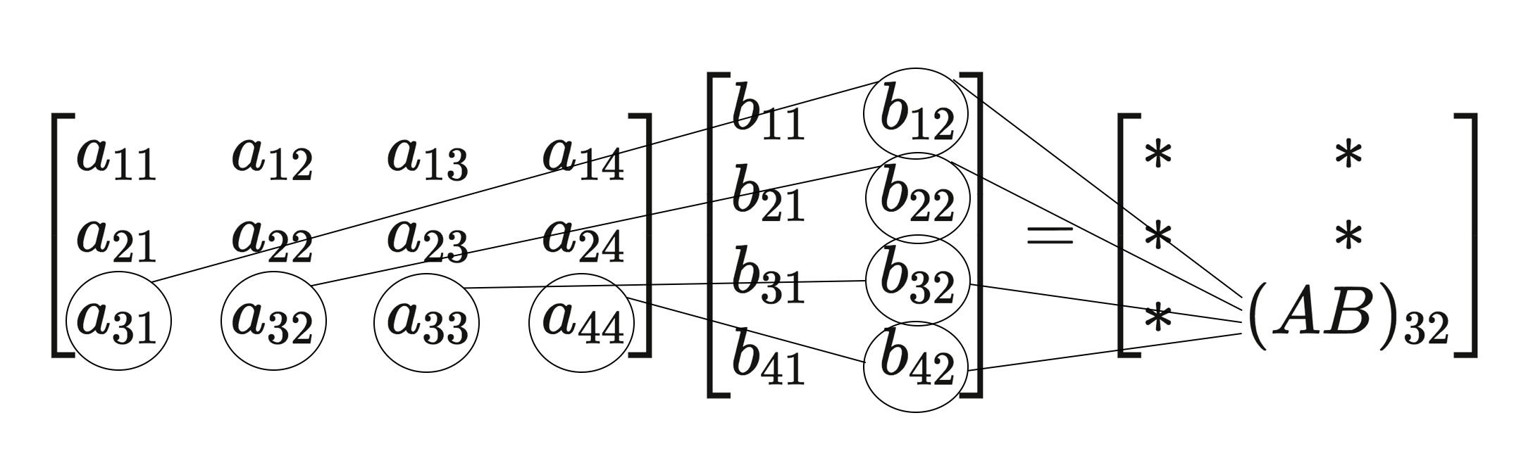
1C The entry \, i, j \, of \, A B \, is the inner product of the \, i \, th row of \, A \, and the \, j \, th column of \, B . For the example in Fig. 1.6,
\, {(A B)}_{32} = a_{31} b_{12} + a_{32} b_{22} + a_{33} b_{32} + a_{34} b_{42} .
///// Fig 1.6. An illustration of matrix multiplication.
\, \begin{bmatrix} a_{11} & a_{12} & a_{13} & a_{14} \\ a_{21} & a_{22} & a_{23} & a_{24} \\ a_{31} & a_{32} & a_{33} & a_{44} \end{bmatrix} \begin{bmatrix} b_{11} & b_{12} \\ b_{21} & b_{22} \\ b_{31} & b_{32} \\ b_{41} & b_{42} \end{bmatrix} = \begin{bmatrix} * & * \\ * & * \\ * & (AB)_{32} \end{bmatrix}
///////
///////
Note. We write \, A B \, when the matrices have nothing special to do with Gaussian elimination. Our earlier example was \, E A , because of the “elementary” matrix \, E ; later it will be \, P A , or \, L U , or even \, L D U . In every case we use the same general rule for matrix multiplication.
EXAMPLE 4
\, A B = \begin{bmatrix} 1 & 0 \\ 2 & 3 \end{bmatrix} \begin{bmatrix} a & b \\ c & d \end{bmatrix} = \begin{bmatrix} a & b \\ 2a + 3c & 2b + 3d \end{bmatrix} .
By columns, this illustrates the property we hoped for. \, B \, consists of two columns side by side, and \, A \, multiplies each of them separately. Therefore each column of \, A B \, is a combination of the columns of \, A . Just as in a matrix-vector multiplication, the columns of \, A \, are multiplied by the individual numbers (or letters) in \, B . The first column of \, A B \, is \, a \, times column 1 plus \, c \, times column 2.
Now we ask about the rows of \, A B . The multiplication can also be done a row at a time. The second row of the answer uses the numbers \, 2 \, and \, 3 \, from the second row of \, A . These numbers multiply the rows of \, B , to give \, 2 \begin{bmatrix} a & b \end{bmatrix} + 3 \begin{bmatrix} c & d \end{bmatrix} . Similarly the first row of the answer uses the numbers \, 1 \, and \, 0 \, to give \, 1 \begin{bmatrix} a & b \end{bmatrix} + 0 \begin{bmatrix} c & d \end{bmatrix} . Exactly as in elimination, where all this started, each row of \, A B \, is a is a combination of the rows of \, B .
We summarize these different ways to look at matrix multiplication.
1D
(i) Each entry of \, A B \, is the product of a row and a column:
\;\;\;\;\;\; {(A B)}_{ij} = \, row \, i \, of \, A \, times column \, j \, of \, B \,
(ii) Each column of \, A B \, is the product of a matrix and a column:
\;\;\;\;\; column \, j \, of \, A B \, = \, A \, times column \, j \, of \, B \,
(iii) Each row of \, A B \, is the product of a row and a matrix:
\;\;\;\;\; row \, i \, of \, A B \, = row \, i \, of \, A \, times \, B \, .
This property is useful in verifying one of the key properties of matrix multiplication. Suppose we are given three matrices \, A, B \, , and \, C , possibly rectangular, and suppose their shapes permit them to be multiplied in that order. The number of columns in \, A \, and \, B \, match, respectively, the number of rows in \, B \, and \, C . Then the property is this:
1E Matrix multiplication is associative: \, (A B) C = A (B C) .
[…]
We want to get on with the connection between matrix multiplication and Gaussian elimination, but there are two more properties to mention first – one property that matrix multiplication has, and another which it does not have. The property that is does possess is:
1F Matrix operations are distributive:
\;\;\;\;\; A (B + C) = A B + A C \, and
\;\;\;\;\; (B + C) D = B D + C D .
Of course the shapes of these matrices must be properly matched – \, B \, and \, C \, have the same shape, so they can be added, and \, A \, and \, D \, are the right size for premultiplication and postmultiplication. The proof of this law is too boring for words.
The property that fails to hold is a little more interesting:
1G Matrix multiplication is not commutative: Usually \, F E \neq E F .
EXAMPLE 5 Suppose \, E \, is the matrix introduced earlier, to subtract twice the first equation from the second – and suppose \, F \, is the matrix for the next step, to add row 1 to row 3:
\;\;\;\;\; E = \begin{bmatrix} 1 & 0 & 0 \\ -2 & 1 & 0 \\ 0 & 0 & 1 \end{bmatrix} \;\;\;\;\;\;\; and \;\;\;\;\;\;\; F = \begin{bmatrix} 1 & 0 & 0 \\ 0 & 1 & 0 \\ 1 & 0 & 1 \end{bmatrix} .
These two matrices do commute:
\;\;\;\;\; E F = \begin{bmatrix} 1 & 0 & 0 \\ -2 & 1 & 0 \\ 1 & 0 & 1 \end{bmatrix} = F E .
That product does both steps – in either order, or both at once, because in this special case the order doesn’t matter.
EXAMPLE 6 Suppose \, E \, is the same but \, G \, is the matrix for the final step – it adds row 2 to row 3. Now the order makes a difference. In one case, where we apply \, E \, and then \, G , the second equation is altered before it affects the third. That is the order actually met in elimination. The first equation affects the second which affects the third. If \, E \, comes after \, G , then the third equation feels no effect from the first. You will see a zero in the \, (3, 1) \, entry of \, E G , where there is a \, -2 \, in \, G E :
\, G E = \begin{bmatrix} 1 & 0 & 0 \\ 0 & 1 & 0 \\ 0 & 1 & 1 \end{bmatrix} \begin{bmatrix} 1 & 0 & 0 \\ -2 & 1 & 0 \\ 0 & 0 & 1 \end{bmatrix} = \begin{bmatrix} 1 & 0 & 0 \\ -2 & 1 & 0 \\ -2 & 1 & 1 \end{bmatrix} \,,
but
\, E G = \begin{bmatrix} 1 & 0 & 0 \\ -2 & 1 & 0 \\ 0 & 1 & 1 \end{bmatrix} \, .
Thus \, E G \neq G E . A random example would almost certainly have shown the same thing – most matrices don’t commute – but here the matrices have meaning. There was a reason for \, E F = F E , and a reason for \, E G \neq G E . It is worth taking one more step, to see what happens with all three elimination matrices at once:
\, G F E = \begin{bmatrix} 1 & 0 & 0 \\ -2 & 1 & 0 \\ -1 & 1 & 1 \end{bmatrix} \, ,
and
\, E F G = \begin{bmatrix} 1 & 0 & 0 \\ -2 & 1 & 0 \\ 1 & 1 & 1 \end{bmatrix} \, .
The product \, G F E \, is in the true order of elimination. It is the matrix that takes the original \, A \, to the upper triangular \, U . We will see it again in the next section.
The other matrix \, E F G \, is nicer, because in that order, the numbers \, -2 \, from \, E , \, 1 \, from \, F , and \, 1 \, from \, G \, were not disturbed. They went straight into the product. Unfortunately it is the wrong order for elimination. But fortunately it is the right order for reversing the elimination steps – which also comes in the next section.
Notice that the product of two lower triangular matrices is again lower triangular.
/////// End of quote from Strang (1986)
/////// Quoting Strang (1986, p. 31):
TRIANGULAR FACTORS AND ROW EXCHANGES
We want to look again at elimination, to see what it means in terms of matrices. The starting point was the system \, A x = b .
\, A x = \begin{bmatrix} 2 & 1 & 1 \\ 4 & -6 & 0 \\ -2 & 7 & 2 \end{bmatrix} \begin{bmatrix} u \\ v \\ w \end{bmatrix} = \begin{bmatrix} 5 \\ -2 \\ 9 \end{bmatrix} = b .
Then there were three elimination steps:
(i) Subtract 2 times the first equation from the second:
(ii) Subtract -1 times the first equation from the third;
(iii) Subtract -1 times the second equation from the third.
The result was an equivalent but simpler system, with a new coefficient matrix \, U :
\, U x = \begin{bmatrix} 2 & 1 & 1 \\ 0 & -8 & -2 \\ 0 & 0 & 1 \end{bmatrix} \begin{bmatrix} u \\ v \\ w \end{bmatrix} = \begin{bmatrix} 5 \\ -12 \\ 2 \end{bmatrix} = c .
The matrix \, U \, is upper triangular – all entries below the diagonal are zero.
The right side, which is a new vector \, c , was derived from the original vector \, b \, by the same steps that took \, A \, into \, U . Thus, forward elimination amounted to:
• Start with \, A \, and \, b \,
• Apply steps (i), (ii), (iii) in that order
• End with \, U \, and \, c .
The last stage is the solution of \, U x = c \, by back-substitution, but for the moment we are not concerned with that. We concentrate on the relation of \, A \, to \, U .
The matrices \, E \, for step (i), \, F \, for step (ii), and \, G \, for step (iii) were introduced in the previous section. They are called elementary matrices, and it is easy to see how they work. To subtract a multiple \, l \, of equation \, j \, from equation \, i , put the number \, -l \, into the \, (i, j) \, position. Otherwise, keep the identity matrix, with \, 1 ‘s on the diagonal and \, 0 ‘s elsewhere. Then matrix multiplication executes the step.
The result of the three steps is \, G F E A = U . Note that \, E \, is the first to multiply \, A , then \, F , then \, G . We could multiply \, G F E \, together to find the single matrix that takes \, A \, to \, U \, (and also takes \, b \, to \, c ). Omitting the zeros it is
\, G F E = \begin{bmatrix} 1 & & \\ & 1 & \\ & 1 & 1 \end{bmatrix} \begin{bmatrix} 1 & & \\ & 1 & \\ 1 & & 1 \end{bmatrix} \begin{bmatrix} 1 & & \\ -2 & 1 & \\ & & 1 \end{bmatrix} = \begin{bmatrix} 1 & & \\ -2 & 1 & \\ -1 & 1 & 1 \end{bmatrix}.
This is good, but the most important question is exactly the opposite: How would we get from \, U \, back to \, A \, ? How can we undo the steps of Gaussian elimination?
A single step, say step (i), is not hard to undo. Instead of subtracting, we add twice the first row to the second. (Not twice the second row to the first!) The result of doing both the subtraction and the addition is to bring back the identity matrix:
\, \begin{bmatrix} 1 & 0 & 0 \\ 2 & 1 & 0 \\ 0 & 0 & 1 \end{bmatrix} \begin{bmatrix} 1 & 0 & 0 \\ -2 & 1 & 0 \\ 0 & 0 & 1 \end{bmatrix} = \begin{bmatrix} 1 & 0 & 0 \\ 0 & 1 & 0 \\ 0 & 0 & 1 \end{bmatrix} .
One operation cancels the other. In matrix terms, one matrix is the inverse of the other. If the elementary matrix E has the number \, -l \, in the \, (i, j) \, position, then its inverse has \, +l \, in that position. That matrix is denoted by \, E^{-1} . Thus \, E^{-1} \, times \, E \, is the identity matrix; that is equation (4).
We can invert each step of the elimination, by using \, E^{-1} \, and \, F^{-1} \, and \, G^{-1} . The final problem is to undo the whole process at once, and see what matrix takes \, U \, back to \, A . Notice that since step (iii) was last in going from \, A \, to \, U , its matrix \, G \, must be the first to be inverted in the reverse direction. Inverses come in the opposite order, so that the second step is \, F^{-1} \, and the last is \, E^{-1} :
\, E^{-1} F^{-1} G^{-1} U = A .
You can mentally substitute \, G F E A \ for \, U , to see how the inverses knock out the original steps.
Now we recognize the matrix that takes \, U \, back to \, A . It has to be \, E^{-1} F^{-1} G^{-1} , and it is the key to elimination. It is the link between the \, A \, we start with and the \, U \, we reach. It is called \, L , because it is lower triangular. But it also has a special property that can be seen only by multiplying it out:
\, \begin{bmatrix} 1 & & \\ 2 & 1 & \\ & & 1 \end{bmatrix} \begin{bmatrix} 1 & & \\ & 1 & \\ -1 & & 1 \end{bmatrix} \begin{bmatrix} 1 & & \\ & 1 & \\ & -1 & 1 \end{bmatrix} = \begin{bmatrix} 1 & & \\ 2 & 1 & \\ -1 & -1 & 1 \end{bmatrix} = L .
Certainly \, L \, is lower triangular, with \, 1 ‘s on the main diagonal and \, 0 ‘s above. The special thing is that the entries below the diagonal are exactly the multipliers \, l = 2, -1 \, and \, -1 . Normally we expect, when matrices are multiplied, that there is no direct way to read off the answer. Here the matrices come in just the right order so that their product can be written down immediately. If the computer stores each multiplier \, l_{ij} \, – the number that multiplies the pivot row when it is subtracted from row \, i , and produces a zero in the \, i, j \, position – then these multipliers give a complete record of the elimination. They fit right into the matrix \, L \, that takes \, U \, back to \, A .